


Model predictive tracking control based on adaptive sliding mode constraints for unmanned underwater vehicles
 0
0 
Abstract
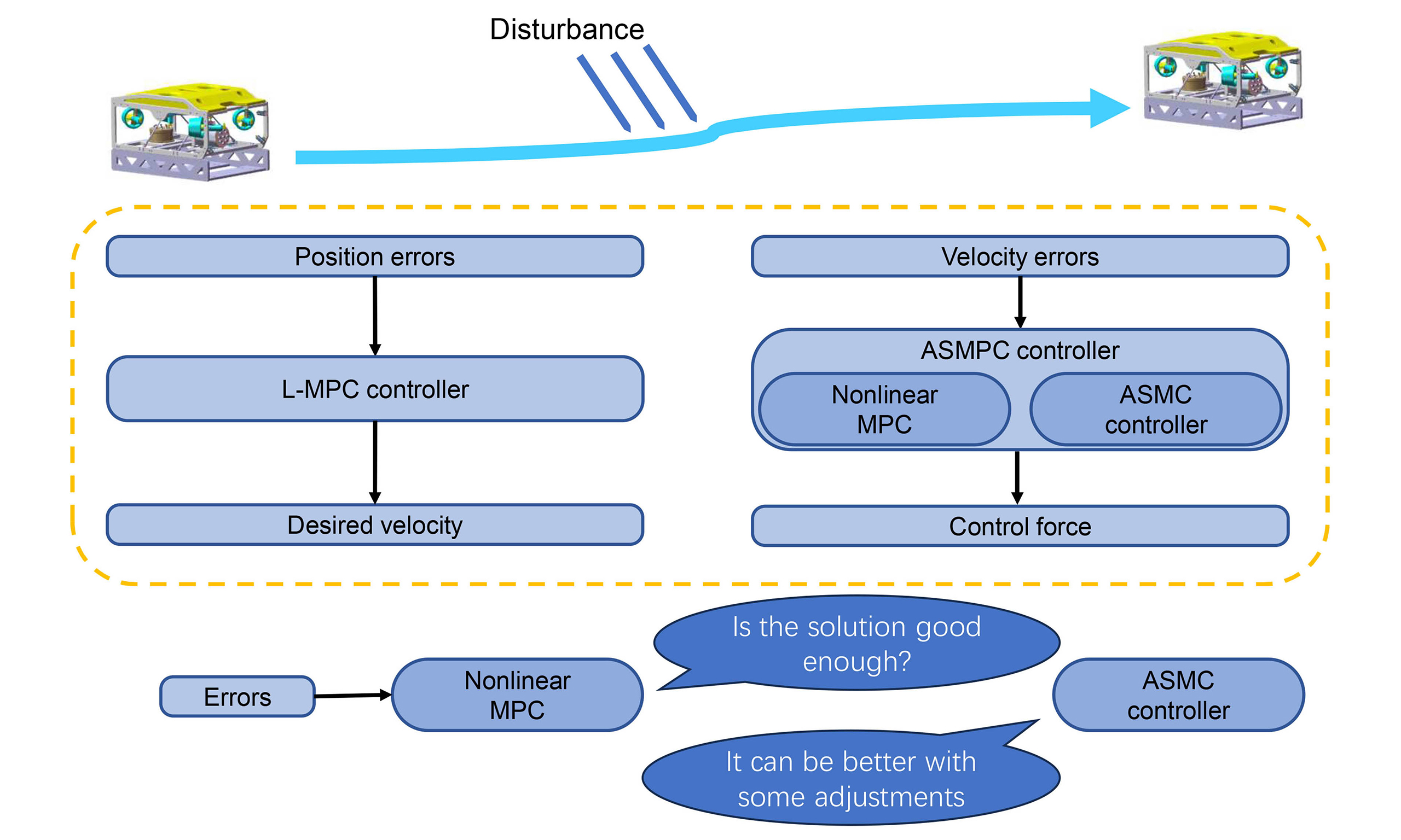
This study presents an improved model predictive control (MPC) approach for unmanned underwater vehicle trajectory tracking, specifically in an environment with ocean current disturbance. The proposed control strategy consists mainly of two MPC frameworks. Each MPC framework additionally attaches a nonlinear constraint used to further optimize the results. The constraint of the first part uses the Lyapunov direct method, while the constraint in the second part is based on the adaptive sliding mode controller, which has a decisive impact on the performance of the whole controller. These constraints give the system the ability to optimize the force output, increase the robustness, and reduce the tracking error. To evaluate the performance of the proposed controller, simulation experiments are conducted, comparing it with commonly used controllers. The results show the characteristics of the proposed method, including stability in the presence of undetectable disturbances and the advantage of effectively mitigating thrust saturation and oscillation caused by motion coupling.
Keywords
1. INTRODUCTION
An unmanned underwater vehicle (UUV) is a highly versatile platform with significant potential for various applications. It can be customized for specific environments[1], featuring diverse structural designs and actuation systems[2]. In practical applications, the automation of the UUV is crucial. This automation includes mission planning, path planning, and trajectory tracking. Trajectory tracking plays a vital role in achieving this automation[3].
UUV is a highly nonlinear system, which presents challenges to control approaches. The effectiveness of trajectory tracking is largely dependent on its accuracy and robustness to disturbance, making the design of robust and high-precision control systems a key area of current research. Several algorithms have been applied to the control of such systems, including proportional-integral-derivative (PID) control[4], sliding mode control[5], reinforcement learning (RL) control method[6], and model predictive control (MPC)[7]. PID control methods have simple structures and low computational complexity. However, it exhibits limited accuracy and robustness when applied to nonlinear systems. It also requires high precision model design control parameters[8]. In contrast, single sliding mode controllers provide high accuracy and robustness in nonlinear system control. Nonetheless, additional control units are typically required to suppress chattering effects, which otherwise compromise control performance[9]. Recently, RL has become a popular research direction. By interacting with a designed environment and updating the policy through trial and error, RL can learn near-optimal control strategies without explicit analytical derivation. The resulting control behavior is adaptive and efficient once training is completed. However, their stability is difficult to establish rigorously, and the training and debugging processes are often complex and time-consuming. Its current applications for the UUV are mostly focused on path planning[10] or actuator-level optimization[11]. MPC is particularly advantageous due to its robustness in handling system uncertainties and external disturbances. Additionally, MPC allows for the incorporation of various constraints during the optimization process[12]. These features allow it to meet practical demands and optimize the output of the control signal. As a result, MPC has been successfully applied in a range of control scenes[13-15]. These studies confirm the feasibility of MPC for engineering practice.
Recently, these methods have been widely used for UUV control. Shen et al. generated B-splines by referring to the current position and the target trajectory to ensure the high-order continuous derivability of the actual trajectory, calculated the kinematic control variables, and then used MPC for dynamic control, which improved the error convergence speed of UUV turning[16]. Shen et al. added variable look-ahead distance parameter based on Line Of Sight (LOS) algorithm to improve overall tracking accuracy[17]. Liang et al. improved the adaptive sliding mode controller and combined it with a PID controller to optimize the convergence speed of the system and improve the stability of each degree of freedom of the underactuated system in the tracking process[18]. The above studies did not deeply discuss the situation of the presence of ocean currents, which is inconsistent with the actual operating environment of UUV and is difficult to use in practical engineering. Some studies have taken this factor into account to investigate the controller performance under current disturbances in depth.
Liang et al. proposed an adaptive disturbance rejection control strategy on UUV to improve robustness and maintain high tracking accuracy in the presence of current disturbance[19]. Yu et al. employed an MPC-based kinematic controller, combined with Fast Integral Terminal Sliding Mode Control (FITSMC) with adaptive control for dynamic control[20]. This method improves the computational efficiency and robustness of the algorithm. Despite the robustness enhancements achieved by these methods, they generally overlook the force limitations imposed by thruster saturation. Once thrust saturation occurs, these controllers may no longer maintain the desired accuracy or robustness.
To address this issue, some studies have proposed targeted improvements to the controllers. Liu et al. adopted a neural network to refine the estimated UUV model in real time, aiming to reduce actuator chattering[21]. Similarly, Guo et al. integrated a nonlinear sliding mode controller within a comparable framework to smooth actuator outputs, though noticeable chattering remained[22]. Other studies have focused on the improvement of MPC controllers. They introduced a constraint-based enhancement to the MPC framework to explicitly account for thruster limitations while improving system robustness. Wei et al. proposed an MPC framework based on Lyapunov constraints, which makes the MPC method globally stable even within a limited number of prediction steps[23]. This constraint is computed online and is fast. However, it is based on the backstepping method, which will produce sudden changes in control force. Gan et al. used Quantum-behaved Particle Swarm Optimization Model Predictive Control (QPSO-MPC) for kinematic control and an adaptive sliding mode controller for dynamic control, which basically eliminated chattering[24].
Motivated by these developments, this paper proposes a constrained double closed-loop feedback system. The system is based on MPC solved by Sequential Quadratic Programming Method (SQP). The dynamic control part is based on the Lyapunov direct method to construct constraints, and the kinematic part is based on the adaptive sliding mode controller to construct constraints. The nonlinear constraints added in this controller are computed online. The main contributions made in this study are as follows:
(1) A constraint based on the adaptive sliding mode controller is integrated into the nonlinear MPC framework to ensure smooth and stable actuation during underwater trajectory tracking. By allowing the auxiliary controller to dynamically adjust the optimization solutions of the MPC, the proposed method effectively mitigates control chattering and maintains a continuous thrust output. This enhances control precision and avoids thrust saturation caused by sudden changes in control input.
(2) An online update strategy of the constraint is established within the system to handle external disturbances. The constraint boundaries are adaptively adjusted in real time according to the predicted system evolution and estimated environmental influences, thereby improving the robustness. These characteristics make it suitable for accurate and reliable trajectory tracking of the UUV.
The remainder of this article is organized as follows. Section 2 covers the dynamic modeling of the UUV, the generation of tracking trajectories, and the implementation of current disturbance. Section 3 describes the design of the trajectory tracking control system based on the Adaptive Sliding Mode Model Predictive Control (ASMPC). Section 4 evaluates the system’s performance through comparative experiments. Finally, Section 5 summarizes the findings and conclusions of the study.
2. PROBLEM FORMULATION
This section introduces the establishment of the UUV trajectory tracking environment. The object of this study is shown in Figure 1, and Table 1 presents the basic information of the platform. The establishment of the coordinates is shown in Figure 2. The body-fixed reference frame O-xyz is defined with the center of the UUV as the origin, and each axis coincides with the principal axis of inertia. The Ox-axis points forward along the longitudinal direction of the UUV, and the Oz-axis points downward along the diving direction. The coordinate system is right-handed, as described in related research[25]. This coordinate system is used to describe the attitude, velocity, and acceleration of the UUV. The position and trajectory information of the UUV is represented by the earth-fixed coordinate system. This coordinate system is right-handed, and the OZ-axis is parallel to gravity. The origin and the other axes of the coordinate system are determined by the specific environment.
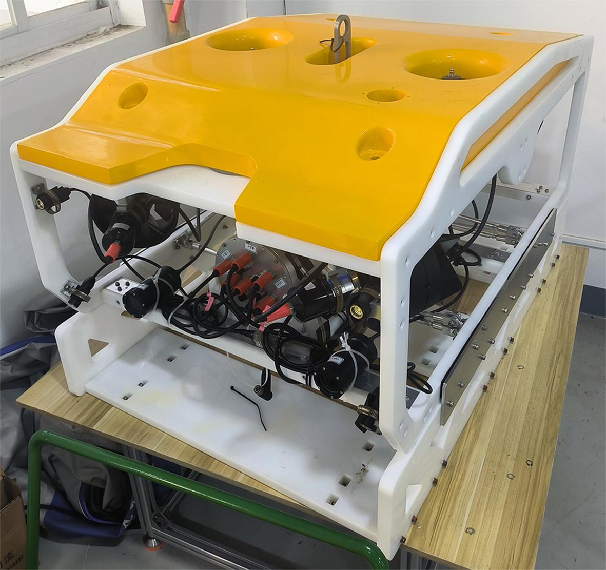
Figure 1. Haixun 2, a Chinese ROV platform serving as the reference model for the simulation experiments in this study. ROV: Remotely operated vehicle.
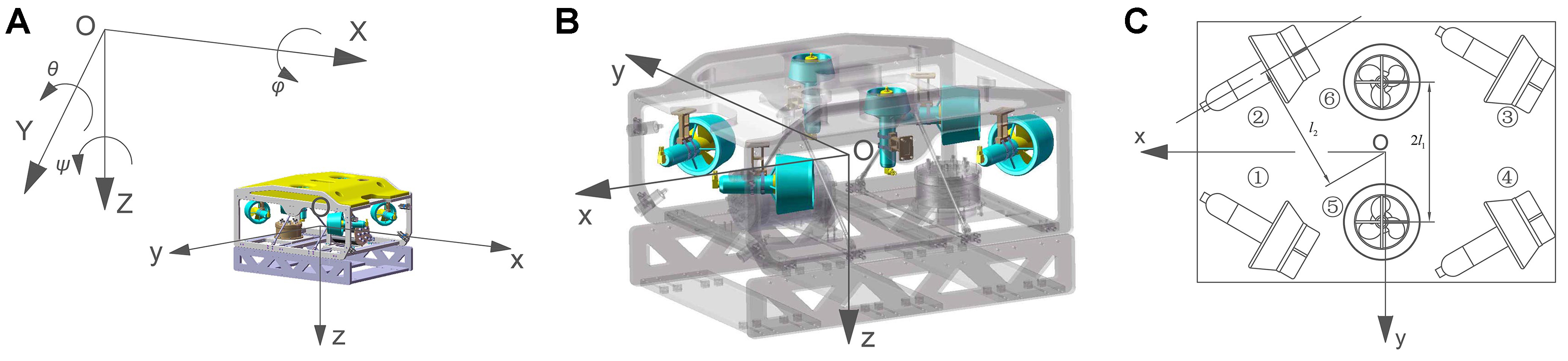
Figure 2. The coordinate systems of the UUV. (A) The earth-fixed and body-fixed coordinate systems; (B) Arrangement of thrusters; (C) The number and exact location of thrusters. UUV: Unmanned underwater vehicle.
Basic parameters of Haixun 2
| Name | Unit | Value |
| Length | m | 1.20 |
| Width | m | 0.85 |
| Height | m | 0.75 |
| Volume | m3 | 0.1162 |
| Weight in air | kg | 116 |
| Maximal speed | knot | 2.5 |
2.1. Kinematics and dynamics of Haixun 2
The spatial position and orientation of the UUV in the earth-fixed coordinate system are expressed by η = [x, y, z, φ, θ, ψ]T, and the velocity and angular velocity in the body-fixed coordinate system on the body are indicated by v = [u, v, w, p, q, r]T. The transformation relationship between the earth-fixed and body-fixed coordinate systems depends on attitude, expressed as
The rotation matrix R(η) and the transformation matrix T(η) are defined as follows:
The dynamics of UUV are characterized by the mass matrix M, the rigid Coriolis force matrix C, the viscous resistance matrix D, the restoring force matrix g, and the resultant force τ as described in[26]. The attitude and velocity dynamics of UUV are governed by
τ = [X, Y, Z, K, M, N]T can be obtained by expanding this equation, where the elements of τ are forces and moments in all directions. This equation intuitively illustrates the coupling process between different motions and the force of the UUV. Leaving x = col(η, v) as the state of the system and u = col(v, τ) as input, the system can be expressed in a general form as
τ in Equation (5) is obtained by synthesizing the thrust generated by each thruster of the UUV. The relevant calculation process is mentioned in the next part.
In the actual operation, the UUV will inevitably encounter a current disturbance. To verify the robustness of the method involved in this study, ocean currents of different intensities are added to the simulation. The added current can be obtained by[27]
In this simulation, let t = 4, c = 1.2, k = 0.5, e = 0.2, b0 = 2.1,
2.2. Thrust allocation
The thruster arrangement is shown in Figure 2. The thrusters are denoted as Ti, i ∈ (1, 2, …, 6), T1, T2, T3, and T4 are arranged horizontally to generate forward thrust and moment. Each thruster is positioned at an angle of α = 30° relative to the Ox-axis. The plane in which these thrusters are located intersects the origin of the body-fixed coordinate system. Since the forward thrust of these thrusters exceeds the reverse thrust, their maximum thrust direction points behind the UUV. Thrusters T5 and T6 are aligned parallel to the Oz-axis and positioned on the left and right sides of the UUV. The plane containing these thrusters also intersects the origin of the body-fixed coordinate system. So, there is T = [T1, T2, T3, T4, T5, T6]T.
The relationship between τ and the individual thrust force T is given by τ = BT in the simulation, where B is the thrust allocation matrix. Since B is typically a singular matrix, its pseudo inverse B+, obtained by decomposition of the singular value, is used for thrust allocation. In Equation (8), l1 represents the distance from the axis aligned with the thrust direction of T1 or T2 to the projection of the mass center. Likewise, l2 denotes the distance from the axis aligned with the thrust direction of the other thrusters to the center of mass. The relevant parameters are given in Figure 2, where l1 = 0.46 m, l2 = 0.265 m, α = 30°.
3. CONTROL SYSTEM
In this study, the constraint based on the Lyapunov direct method and adaptive algorithm is added to the nonlinear MPC. Before the interpretation of the controller, an assumption about the waypoints is made to ensure the stability of the system.
Assumption 1 The desired reference trajectory ηd is continuous and differentiable up to the required order, and its time derivatives are bounded. This assumption guarantees that the reference signal can be predicted within each sampling interval.
The control block diagram is shown in Figure 3. The system consists of an outer-loop and an inner-loop, which use Lyapunov Direct Method Model Predictive Control (L-MPC) and ASMPC, respectively. The outer-loop considers the position and attitude of the UUV as the system state, with velocity and angular velocity in the earth-fixed frame serving as control inputs. Its objective is to generate a desired velocity that drives the position and attitude errors toward 0. The inner-loop takes the desired velocity as the system state and the total forces and moments as control inputs, aiming to produce control forces that drive the actual velocity to converge to the desired velocity. The main steps of each loop include obtaining the state error, constructing the Lyapunov function, ensuring its asymptotic stability, obtaining the optimization result of the cost function under the constraint, and getting the output of MPC. The system remains asymptotically stable when the controller output follows the control law.
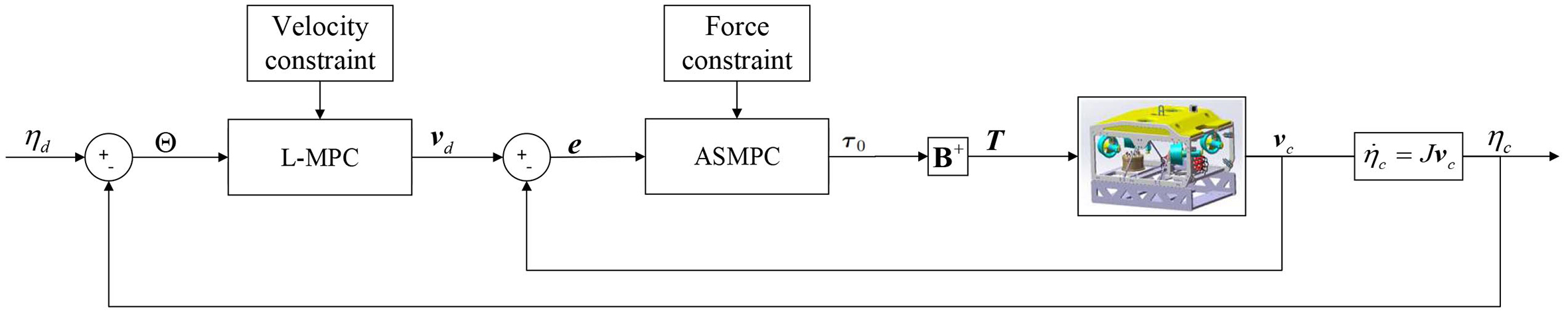
Figure 3. Framework of the system. vd and τ0 are the results of MPC. The Velocity constraint block consists of Equations (14d) and (14e), and the Force constraint block consists of Equations (25d) and (25e). MPC: Model predictive control.
3.1. Kinematic control
The input of the outer-loop control system is the real-time position error. Define the desired state and the actual state of the UUV as ηd and ηc, respectively. Then get the current state of the UUV error Θ = ηd - ηc. The input of the kinematic control is η and the output is v. The kinematic part Equation (5) is then time-discretized and solved:
where each step k represents a predicted time step, and F(·) represents the discrete kinematic function. For a prediction horizon totaling N steps, the sequence of states and controls can be written as
The nonlinear MPC calculation process involves predicting the error of N waypoints, so
Then, the nonlinear MPC control problem in path tracking can be obtained as
Here, η0 is the initial value. vmax is the velocity limitation of the UUV. Q1, R1, and P1 are positive definite weight matrices.
In the trajectory tracking problem, the number of predicted steps cannot cover the whole trajectory. Especially when there is external interference, the optimal solution is unable to guarantee closed-loop stability[29]. To ensure that the optimization results lead to asymptotic stability of the system, a Lyapunov-based control design is incorporated into the formulation. According to[30], this control law will be added in the form of an additional constraint
where f(·) is the undiscretized system, V1(·) is the constructed Lyapunov function and h1(·) is the selected nonlinear control law. Referring to[31], it will be solved by SQP. In the process of solving, the control sequence U = [vkT, …, vk+N-1T]T is collected as the decision variable and the predicted states ηk+i are calculated by the changes, denoted by Δηk+i and Δvk+i. At each iteration, represented by j, the kinematics and nonlinear constraints are linearized about the current nominal trajectory:
with Ai(j) = ∂f/∂η, Bi(j) = ∂f/∂v evaluated at the nominal. Using these sensitivities, a quadratic programming (QP) subproblem is formed:
where H(j) is the second order gradient of current cost assembled using a Gauss–Newton approximation, λ(j) is the current cost gradient, c(·) denotes the hard constraint, and Jc(j) contains the contraction constraint. After several SQP iterations to make ΔU small enough, only vk is applied and the horizon is shifted for the next step.
The new constraint Equation (14e) added to the control problem enables the final optimization result to inherit the stability of the controller h1. The calculation process for this constraint is online and complies with other constraints set in the system. In this section, a first-order system needs to be controlled and the controller h1 is designed by the Lyapunov direct method. Consider the following Lyapunov function:
where K1 is a positive definite gain matrix. Then taking the derivative of V1 with respect to the state, there is
Define the velocity control law as
where Kp is a positive definite gain matrix. Note that v here is the value used by the algorithm to compute the constraint Equation (14e) and is not directly related to the output v1 of the controller.
Then there is
In summary, the essence of the method is to obtain the possible suboptimal solution of MPC by establishing an additional constraint. The study[30] names this additional constraint the contraction constraint and proves its superiority in guaranteeing the stability of the system. Therefore, this suboptimal solution is perfectly acceptable in the system.
3.2. Dynamic control
The inner-loop control system is designed to ensure stable thruster force output that drives the UUV velocity error e = vd - vc to converge to 0, where vd is provided by the outer-loop control and vc is the real velocity of the UUV. The dynamic part in Equation (5) is time-discretized and solved:
and the sequence of states and controls in the prediction process is written as
The error
Similar to the outer-loop, the inner-loop control problem can then be formulated as the following optimal control problem with contraction constraints:
where Q2, R2, and P2 are also positive definite weight matrices, τmax is the thrust limitation of the UUV. It will be solved by SQP with a similar solving process in the kinematics section. A nonlinear controller h2(·) will also be added to the optimization process in the form of contraction constraint Equation (25e). According to Equation (14d), vd is bounded, and the real velocity vc of the UUV is also bounded. Obviously, the input e of the controller can be proved to be bounded, satisfying the condition of using the sliding mode controller. Referring to the controller in the relevant research, the sliding mode surface is defined as[24]
where Λ is a constant.
Choose the force control law as
where
Chattering also occurs when nonlinear constraints based on sliding mode controllers are used. To avoid this problem, an adaptive control law needs to be added. Note that τ here is the value used by the algorithm to compute the constraint Equation (25e) and is not directly related to the output τ0 of the controller. Rewrite the control law as
where Ф(
Construct the following Lyapunov function as
where
Equation (32) is obtained from the definition of S,
Substituting Equation (4) into Equations (32) and (33), make the following transformation
Substitute Equation (28) in, there is
where
According to Equation (25), the complete form of the nonlinear constraint is constructed as
The actual dynamic model terms can be cancelled out during computation, and this constraint can be reformulated into the structure of Equation (39). As a result, the constraint introduces minimal computational overhead, while retaining its optimization benefits.
Then the detailed form of the contraction constraint Equation (25e) of the force control can be obtained as
After the solution is calculated, the force output of each thruster is obtained by T = B+τ0. The control algorithm for ASMPC is summarized in Algorithm 1.
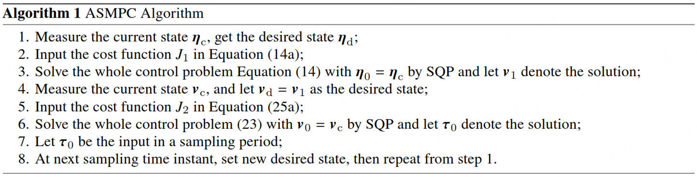
Algorithm 1.
To demonstrate the effectiveness of the proposed controller, two representative MPC variants are implemented for comparison. Robust Model Predictive Control (RMPC) is a conventional worst–case robust formulation, where all possible disturbances within a bounded set are considered in the optimization. The resulting control policy guarantees constraint satisfaction under all admissible uncertainties but tends to be conservative. Stochastic Model Predictive Control (SMPC) is a probabilistic MPC scheme following the stochastic error inheritance, where disturbances are usually modeled as Gaussian random variables and constraints are satisfied with a predefined confidence level. This approach improves average performance but relies on accurate statistical characterization of the uncertainties. In some cases, behavior beyond the constraints is allowed under the method.
In the process of computing ASMPC, the constraint τ0 ∈ U = {τk | |τk| ≤ τmax} must be satisfied. Similarly, h2(·) ∈ U = {τk | |τk| ≤ τmax} is satisfied. According to Equation (39), the range of τ0 is contained within h2(·) and can therefore be redefined as τ0 ∈ UASMPC
4. SIMULATION RESULTS
This section presents the simulation results to demonstrate the effectiveness of the proposed control system. All simulations are based on the model of Haixun 2. The actual initial position of the UUV is set to [0, 0, 0, 0, 0, π/4]T. Assume that the desired trajectory is xd =25sin(2t), yd =25sin(t), zd =22.5 - 12.5sin(t), ψd = arctan(yd/xd), φd = θd = 0. To evaluate the precision and robustness of the proposed method, simulations are conducted in still water and in the presence of current disturbance. The environmental disturbance is assumed to be spatially consistent at different depths for the same location. The detailed simulation parameters are listed in the Supplementary Materials.
Due to the power limitations of the UUV, the thrust of the thrusters is restricted within a reasonable range during the simulation. Specifically, the maximum thrust for the horizontally arranged thrusters T1 to T4 is 170 N in the positive direction and 100 N in the negative direction. For vertically arranged thrusters T5 and T6, the maximum thrust is capped at 100 N in both positive and negative directions. Furthermore, the position and attitude data of the UUV are assumed to be accurately obtained after sensor processing and filtering, ensuring reliable state estimation for trajectory tracking.
The UUV in this study has a 5 degrees-of-freedom (5-DOF) design, and direct angular control over the Oy-axis in the body-fixed reference frame is not feasible. When the UUV moves forward, it generates a moment in the negative direction of the Oy-axis. To mitigate the resulting tracking error in θ and z, thrusters T4 and T5 provide upward thrust to counteract this effect.
4.1. Tracking performance
In this section, a simulation environment with a total length of approximately 242 m, free from disturbance, is established to assess the performance of the system. RMPC and SMPC are added to provide a comparative evaluation. In this simulation, the maximum speed of the UUV is set to 2.5 knots. The desired trajectory and simulation results in still water are presented in Figure 4. Despite operating at the maximum design speed, all three methods successfully track the desired trajectory, further demonstrating the closed-loop stability of the ASMPC.
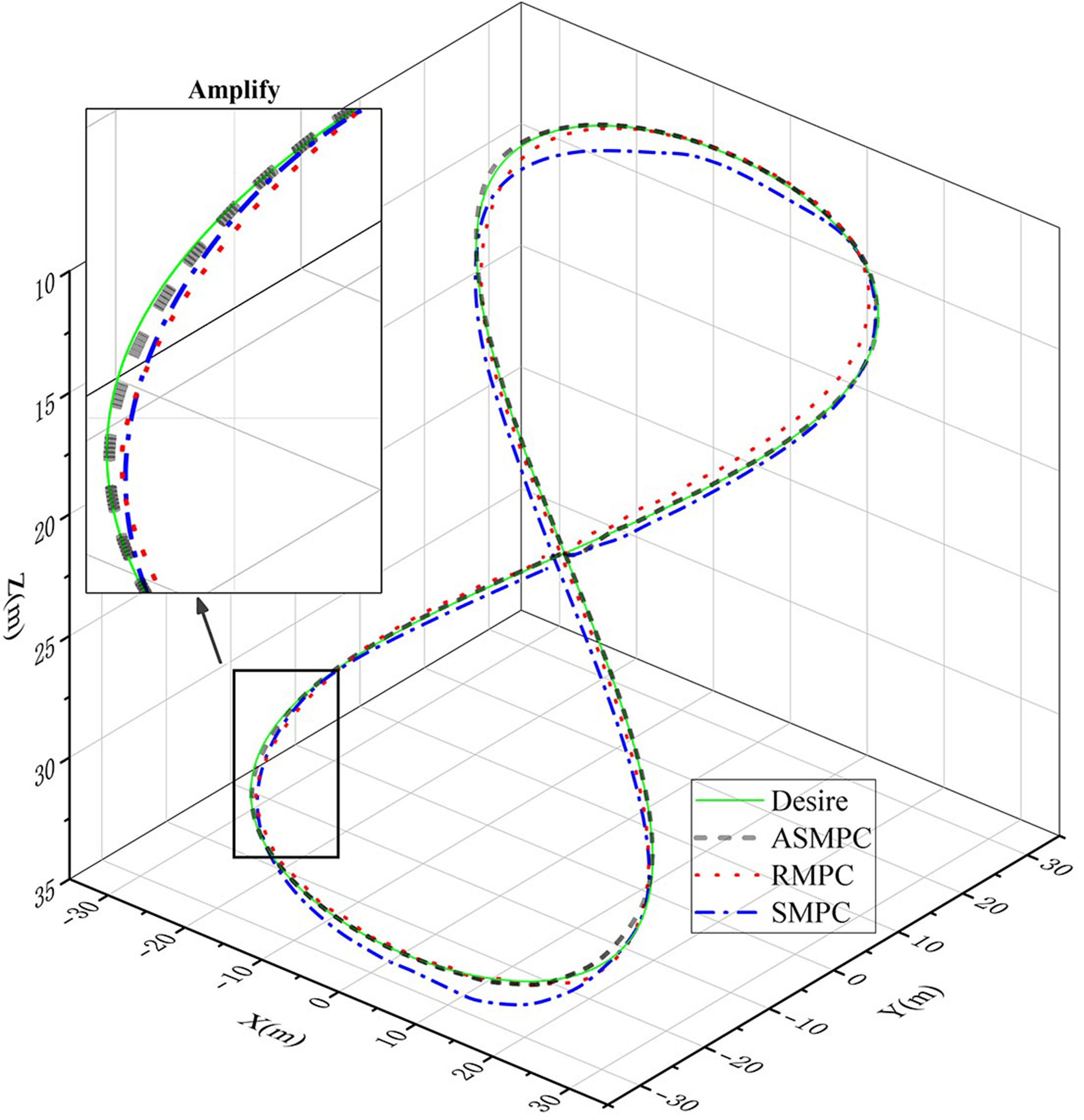
Figure 4. Simulation result of each method without current disturbance.
To evaluate tracking performance, the tracking error is shown in Figure 5. Primary errors occur along the OX-axis and the OZ-axis. Compared to the other two methods, ASMPC exhibits lower error magnitudes and reduced oscillations along all axes, highlighting its superior trajectory tracking accuracy. The angular errors in φ, θ, and ψ are also shown in Figure 5. The UUV utilizing ASMPC maintains stable tracking performance with minimal angular error fluctuations and no divergence tendencies. A noticeable divergence trend in the φ-axis error appears in the RMPC simulation after the 150th s, which corresponds to a sudden increase in the OX-axis error. This indicates a critical performance deficiency of the RMPC controller and confirms the correlation between angular errors and position errors.
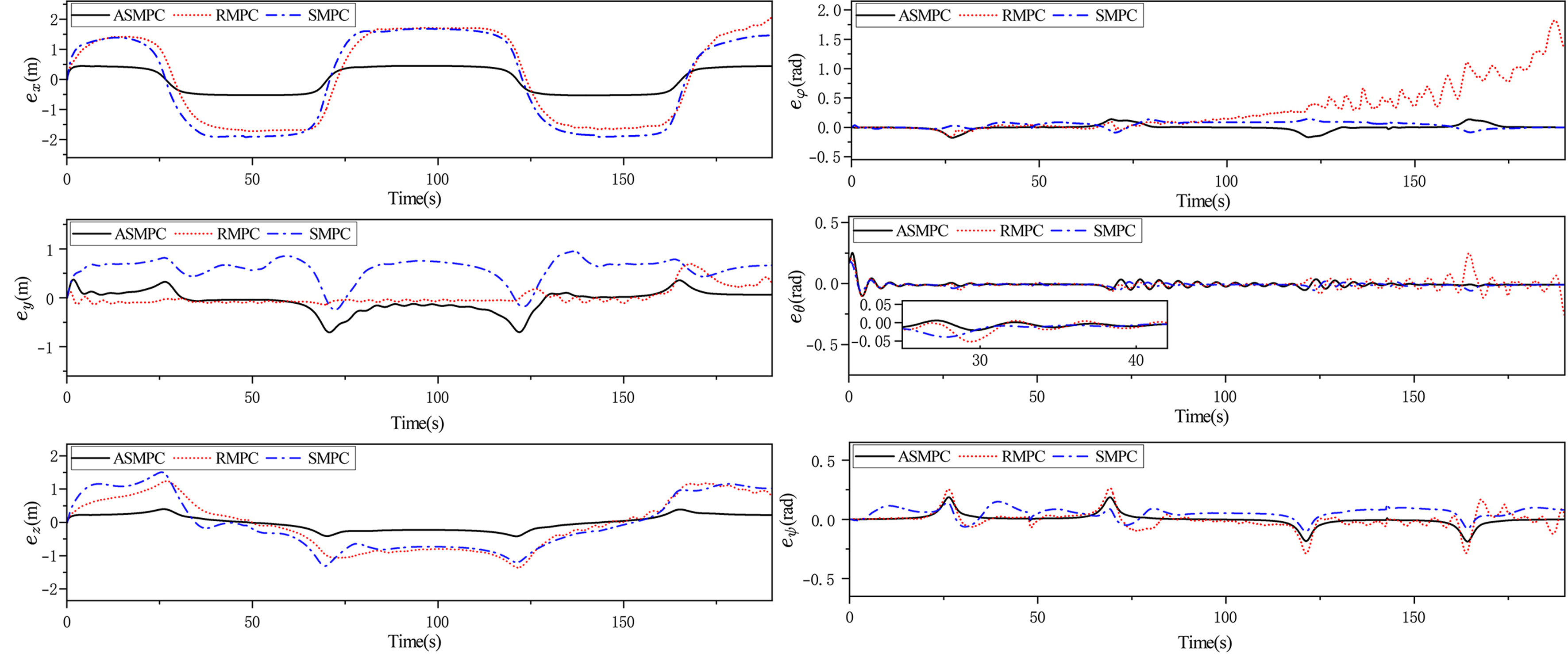
Figure 5. The tracking error and angular error of OX-axis, OY-axis and OZ-axis without current disturbance.
The root mean square errors (RMSE) for this case are summarized in Figure 6. Roughly, the RMSE of ASMPC on position control is at least 3 times smaller than that of other methods. Its RMSE on angular control is also improved compared with other methods.
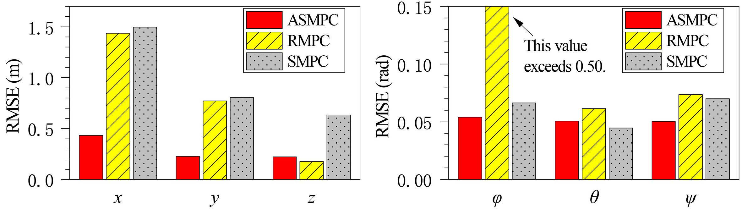
Figure 6. The RMSE in each axis. RMSE: Root mean square errors.
The actual thrust of each thruster is illustrated in Figure 7. The output thrust of each method is within the thrust range. Therefore, the thrust constraint can be considered to be in effect. To achieve a stable control effect, the thrust curve should be as low as possible. ASMPC achieves a more stable thrust output and avoids thrust saturation. In contrast, RMPC exhibits significant oscillations and experiences thrust saturation. This is because the thrust obtained by its solution is much larger than the thrust limit, which also contributes to unacceptable tracking error. Although the SMPC demonstrates slightly lower thrust output, its tracking performance is inferior. This is because SMPC allows for controlled deviations within predefined conditions. In summary, ASMPC demonstrates superior tracking performance in still water, ensuring more stable thrust allocation and reducing the risk of saturation-related performance degradation.
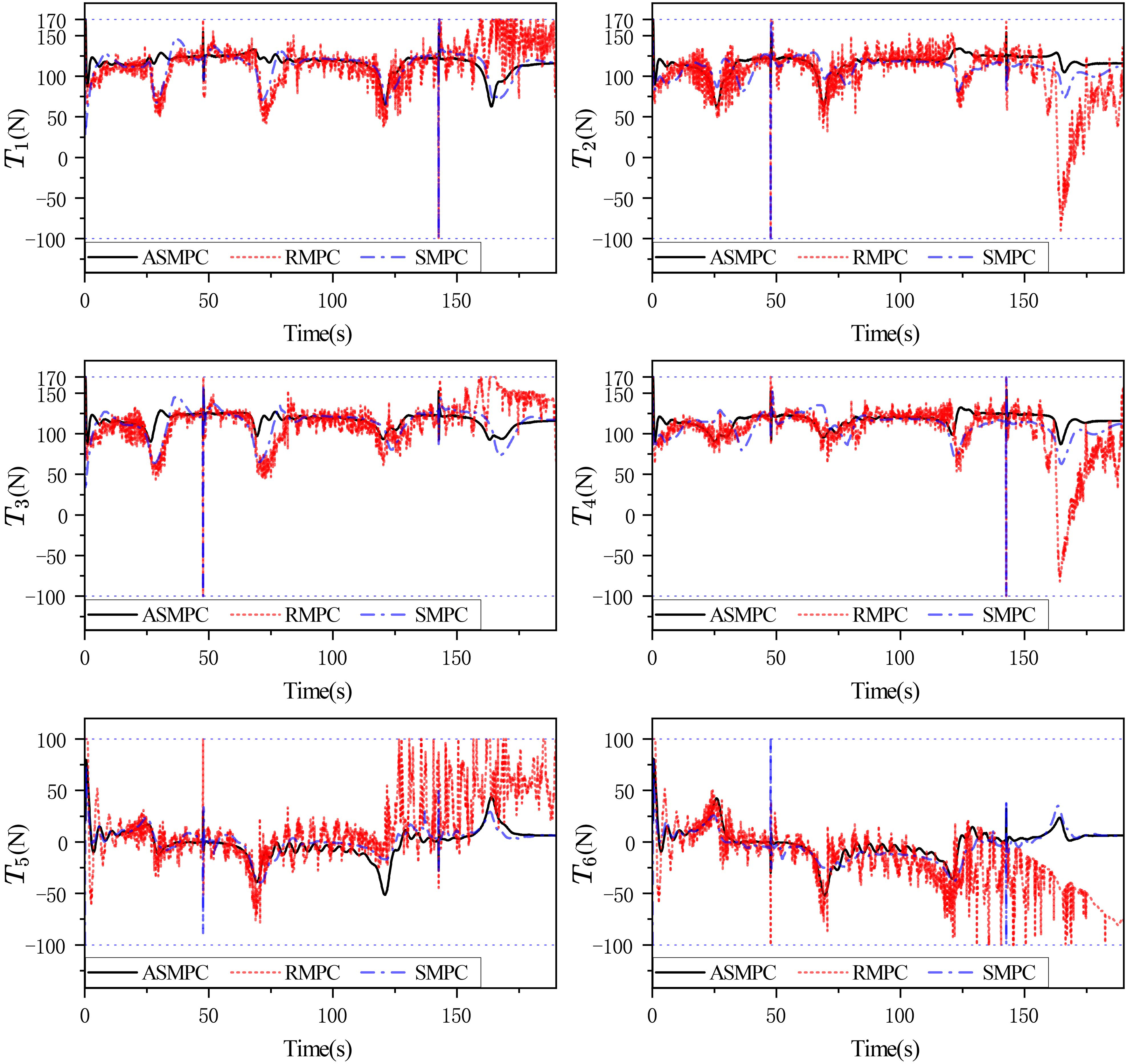
Figure 7. The force generated by each thruster without current disturbance. The set thrust limits have been marked by dashed lines.
4.2. Robust result
In this section, the UUV is required to track the same trajectory in the presence of current disturbance, the desired trajectory, and simulation results are presented in Figure 8. The disturbance is defined by Equations (6) and (7) with a maximum velocity of 0.2 m/s, which is shown in Figure 9. The red arrow indicates the direction of the current at the location, and the arrow length indicates the relative strength of the disturbance. The blue markers indicate the simulation moments corresponding to the two waypoints. Since the disturbance condition is undetectable to the UUV, tracking performance depends on the robustness of the controller itself.
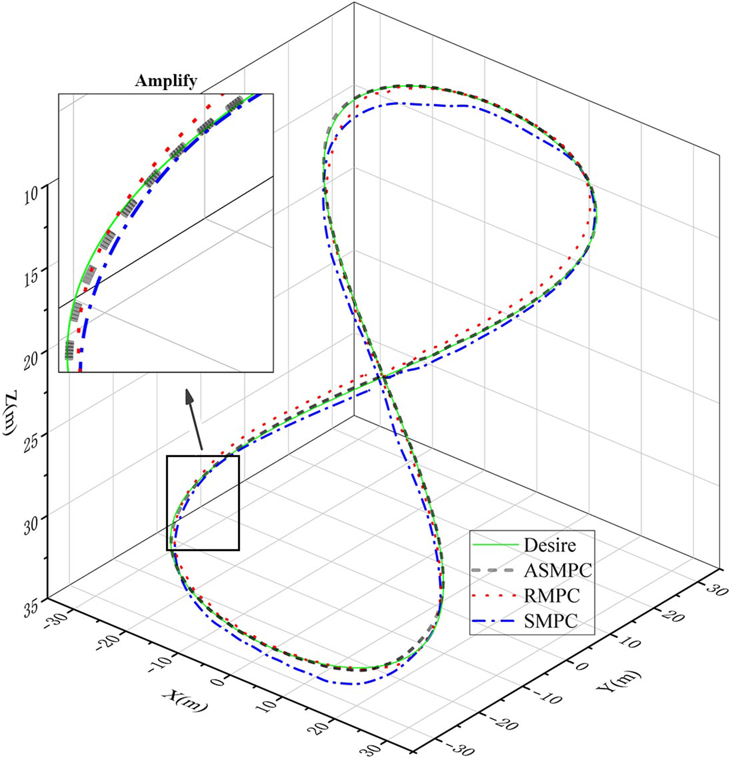
Figure 8. Simulation result of each method with current disturbance.
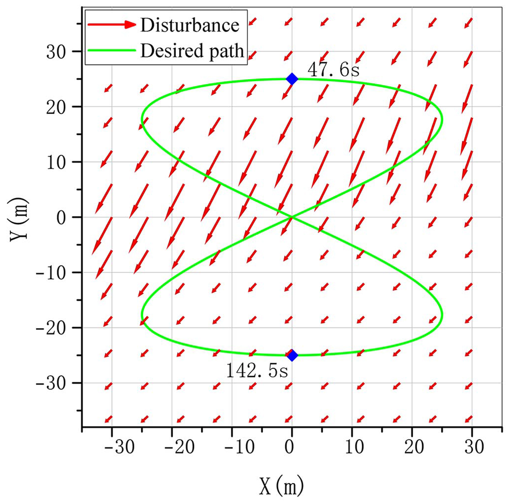
Figure 9. Top view of current disturbance and the desired path.
The tracking error and the angular error for each method are shown in Figure 10. The trend of tracking error in this case follows a pattern similar to that observed in still water. Under disturbance, the tracking error increases across all methods, and the ASMPC method still demonstrates superior tracking accuracy. For the angular error, the disturbance amplifies the oscillations in θ. The RMSEs are summarized in Figure 11. In this case, the RMSE of all parameters in the ASMPC method has no significant increase. This demonstrates the robustness of this constraint under variable disturbances.
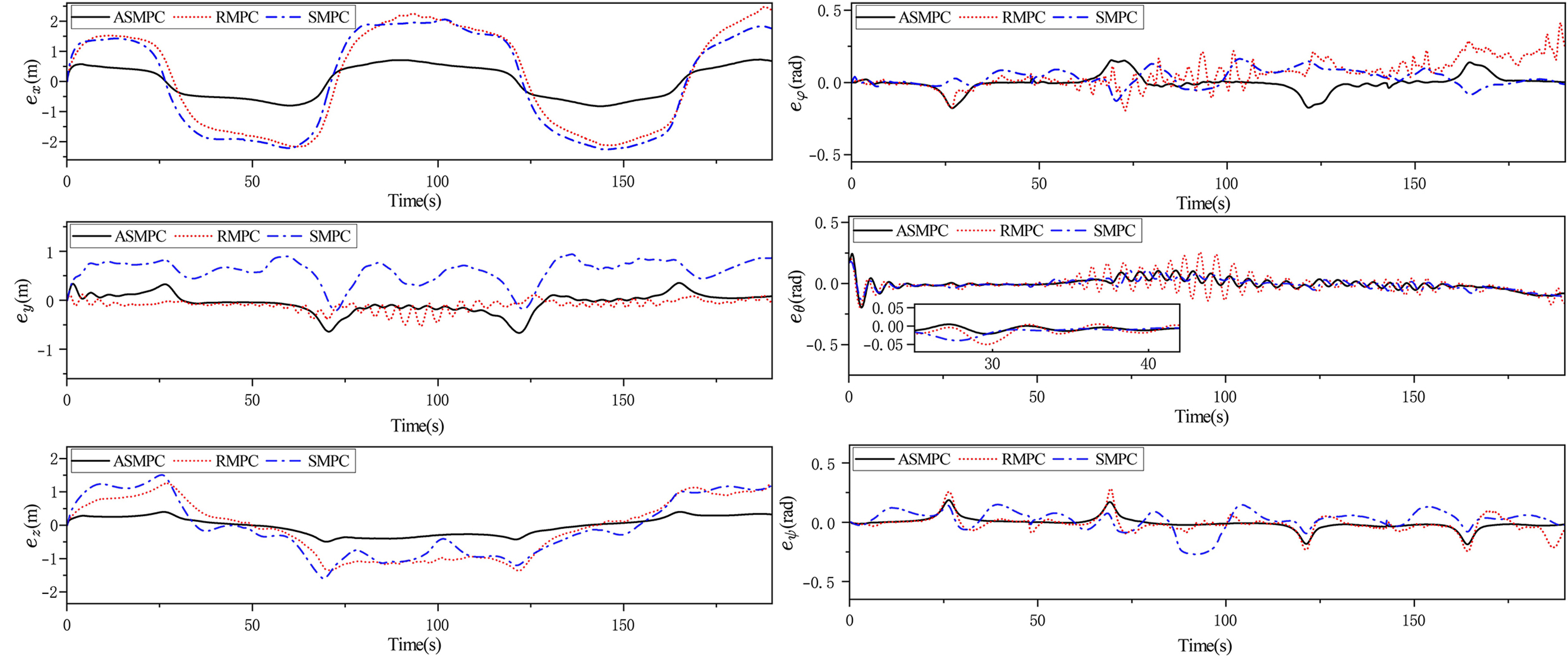
Figure 10. The tracking error and angular error of OX-axis, OY-axis and OZ-axis with current disturbance.
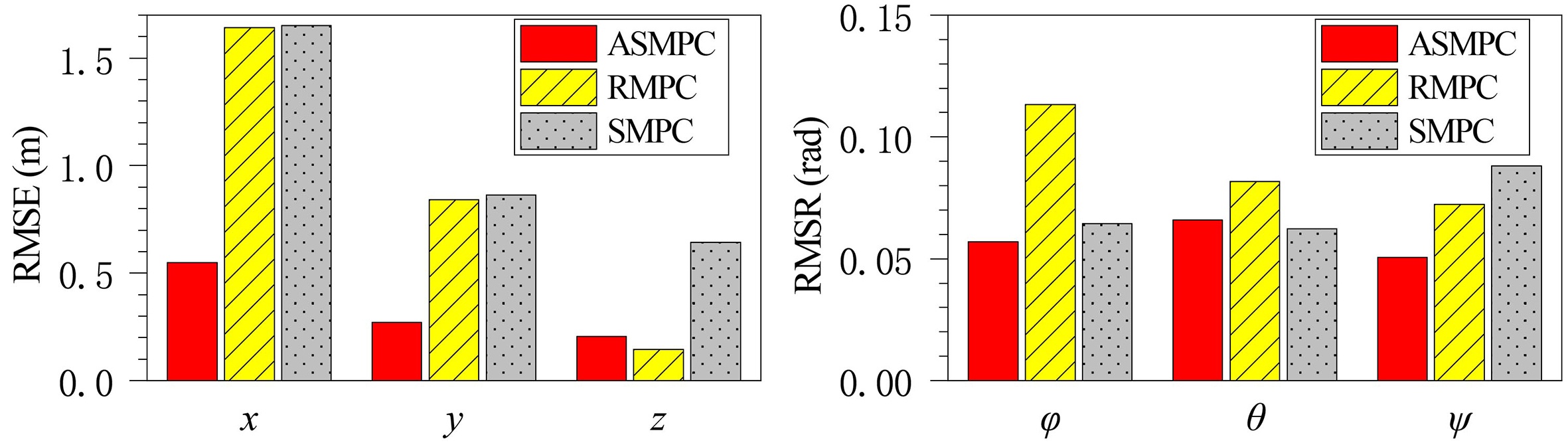
Figure 11. The RMSE in each axis. RMSE: Root mean square errors.
The planned thrust force is shown in Figure 12. Under disturbance, thrust saturation occurs in both the RMPC and the SMPC. T5 and T6 under the control of RMPC experience the most severe oscillation. The situation of SMPC is slightly better; thrust saturation is observed mainly in T2 and T4, and the thrust output is noticeably more stable compared to RMPC. In contrast, ASMPC demonstrates significantly superior thrust control, effectively mitigating thrust saturation, and ensuring stable thrust output. This highlights the high robustness of the ASMPC method.
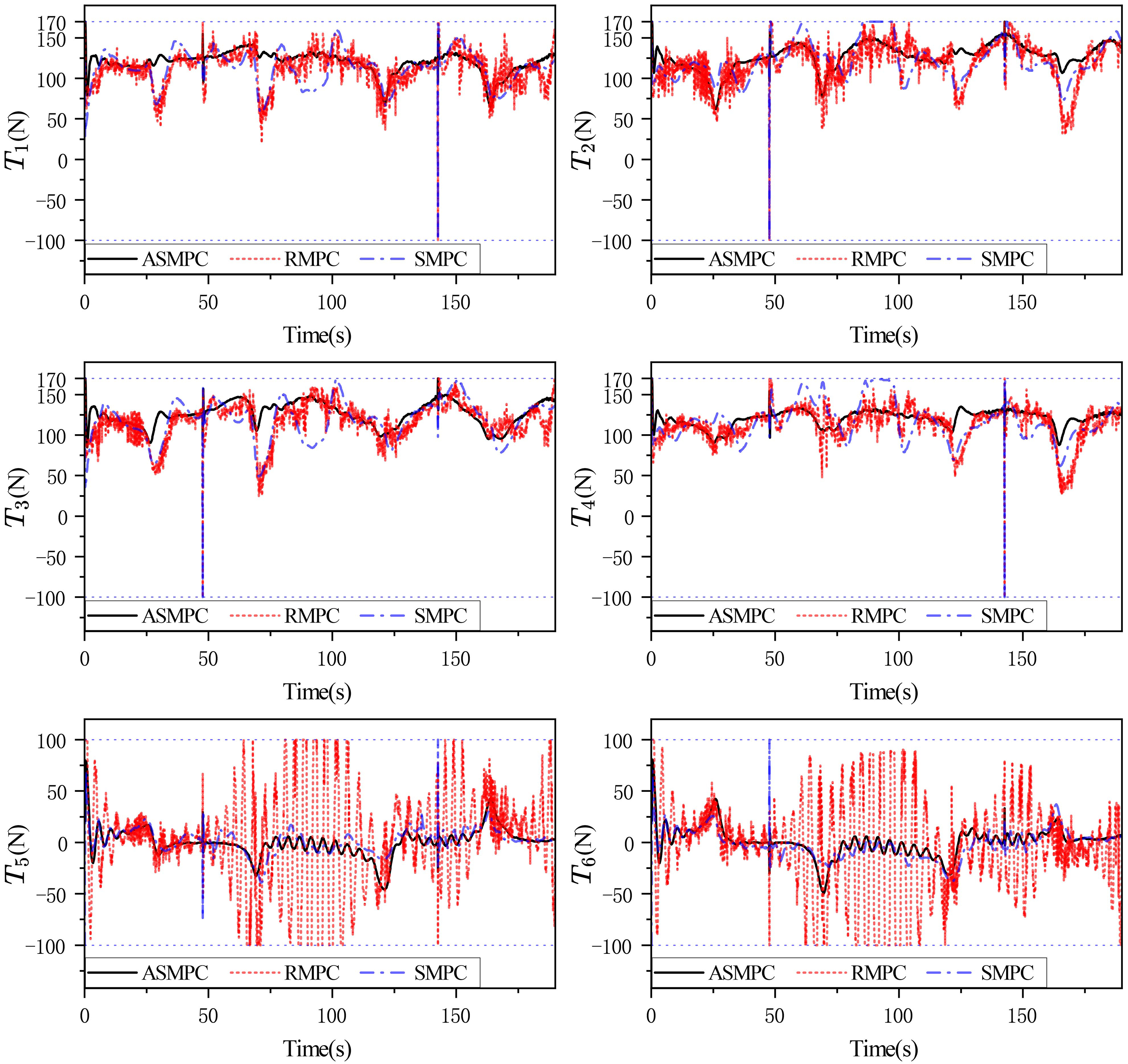
Figure 12. The force generated by each thruster with current disturbance.
5. CONCLUSION
In this study, a control method for UUV trajectory tracking is improved, which is able to adapt to changing current disturbance in trajectory tracking. The convergence of the algorithm is discussed by the Lyapunov stability theorem, and the stability of the system is proved when the system input satisfies the contraction constraint.
The system is capable of tracking complex trajectories, resisting disturbance during the tracking process, and maintaining robust tracking performance under disturbance when the speed reaches the design index. The current disturbance applied in this study is particularly harsh for this UUV design, highlighting the robustness of the proposed method. Compared with the two similar controllers, the proposed method effectively mitigates thrust saturation by constructing stricter constraints, providing the UUV with improved energy efficiency and a more redundant driving allocation strategy.
In future work, the algorithm should be applied to the UUV experiment to verify its trajectory tracking effect in practical use, and the relationship between attitude and tracking error should be further discussed. In addition, measurement errors will inevitably be introduced in the experiment.
DECLARATIONS
Acknowledgments
The authors thank University of Shanghai for Science and Technology and OriginLab for providing the Free OriginPro Learning Edition.
Authors’ contributions
Made substantial contributions to conception and design of the study and performed data analysis and interpretation: Zhang, Y.
Performed data acquisition and provided administrative, technical, and material support: Zhu, D.; Chen, M.
Made substantial contributions to the research and idea generation: Yang, S. X.
Availability of data and materials
The original contributions presented in this study are included in the article/Supplementary Materials. Further inquiries can be directed to the corresponding author.
AI and AI-assisted tools statement
Not applicable.
Financial support and sponsorship
This work was supported in part by the National Natural Science Foundation of China (Grants 52431012 and 62033009), and in part by the Creative Activity Plan for Science and Technology Commission of Shanghai (Grants 23550730300 and 24510712400).
Conflicts of interest
Yang S. X. serves as the Editor-in-Chief of Intelligence & Robotics, and Zhu D. serves as the Section Editor for Robot Control and Navigation in Intelligence & Robotics. Neither of them is involved in any part of the editorial process for this manuscript, including reviewer selection, manuscript handling, or decision-making. The other authors declare no conflicts of interest.
Ethical approval and consent to participate
Not applicable.
Consent for publication
Not applicable.
Copyright
© The Author(s) 2026.
Supplementary Materials
REFERENCES
1. Kim, J. Surface tracking controls of an unmanned underwater vehicle with fixed sonar ray measurements in tunnel-like environments. J. Intell. Robot. Syst. 2024, 110, 29.
2. Zhou, X.; Chen, W.; Li, K.; et al. A 7 cm-scale spherical underwater robot using piezoelectric double-jet actuator for deep-sea environment. IEEE/ASME. Trans. Mechatron. 2024, 29, 3277-88.
3. Zhang, J.; Xiang, X.; Zhang, Q.; Tao, B. Electromagnetic localization and tracking control of underactuated autonomous underwater vehicle for subsea cable detection. IEEE. Trans. Veh. Technol. 2024, 73, 18283-93.
4. Sun, B.; Cui, K.; Wang, P.; Xie, M.; Gao, S.; Cheng, S. A lateral and longitudinal control method based on linear quadratic regulator for intelligent vehicles considering future path changes. Meas. Sci. Technol. 2024, 36, 015103.
5. Wang, Q.; Wang, W.; Suzuki, S.; Namiki, A.; Liu, H.; Li, Z. Design and implementation of UAV velocity controller based on reference model sliding mode control. Drones 2023, 7, 130.
6. Li, X.; Geng, L.; Liu, K.; Zhao, Y.; Du, W. Motion control of autonomous underwater vehicle based on physics-informed offline reinforcement learning. Ocean. Eng. 2024, 313, 119432.
7. Hailong, H.; Eskandari, M.; Savkin, A. V.; Ni, W. Energy-efficient joint UAV secure communication and 3D trajectory optimization assisted by reconfigurable intelligent surfaces in the presence of eavesdroppers. Def. Technol. 2024, 31, 537-43.
8. Tong, L.; Cui, D.; Wang, C.; Peng, L. A novel zero-force control framework for post-stroke rehabilitation training based on fuzzy-PID method. Intell. Robot. 2024, 4, 125-45.
9. Xiao, H.; Zhao, D.; Gao, S.; Spurgeon, S. K. Sliding mode predictive control: a survey. Annu. Rev. Control. 2022, 54, 148-66.
10. Jetto, L.; Orsini, V.; Romagnoli, R. A new approach to model predictive control based on two degrees of freedom control and B-splines input shaping. IEEE. Trans. Autom. Control. 2021, 66, 2770-7.
11. Gao, J.; Li, Y.; Chen, Y.; He, Y.; Guo, J. An improved SAC-based deep reinforcement learning framework for collaborative pushing and grasping in underwater environments. IEEE. Trans. Instrum. Meas. 2024, 73, 1-14.
12. Cannon, M.; Cheng, Q.; Kouvaritakis, B.; Raković, S. V. Stochastic tube MPC with state estimation. Automatica 2012, 48, 536-41.
13. Cao, X.; Ren, L.; Sun, C. Dynamic target tracking control of autonomous underwater vehicle based on trajectory prediction. IEEE. Trans. Cybern. 2023, 53, 1968-81.
14. Song, C.; Zhang, X.; She, Y.; Li, B.; Zhang, Q. Trajectory planning for UAV swarm tracking moving target based on an improved model predictive control fusion algorithm. IEEE. Internet. Things. J. 2025, 12, 19354-69.
15. Marques Barbosa, F.; Löfberg, J. Exponential cone approach to joint chance constraints in stochastic model predictive control. Int. J. Control. 2025, 98, 3024-34.
16. Shen, C.; Shi, Y.; Buckham, B. Model predictive control for an AUV with dynamic path planning. 2015 54th Annual Conference of the Society of Instrument and Control Engineers of Japan (SICE); 2015 Jul 28-30; Tokyo, Japan. IEEE; 2015. pp. 475-80.
17. Shen, G.; Zhou, Z.; Xia, C.; Xu, X.; He, B.; Shen, Y. Path tracking of AUV based on improved line-of-sight method. OCEANS 2022, Hampton Roads; 2022 Oct 17-20; Hampton Roads, USA. IEEE; 2022. p. 1-5.
18. Liang, J.; Liang, J.; Huang, W.; Zhou, F.; Lin, G.; Su, Z. Robust nonlinear path-tracking control of vector-propelled AUVs in complex sea conditions. Ocean. Eng. 2023, 274, 113923.
19. Liang, X.; Qu, X.; Hou, Y.; Li, Y.; Zhang, R. Finite-time unknown observer based coordinated path-following control of unmanned underwater vehicles. J. Franklin. Inst. 2021, 358, 2703-21.
20. Yu, L.; Qiao, L.; Shen, C. Obstacle avoidance for a large-scale high-speed underactuated AUV in complex environments. IEEE. Trans. Intell. Transp. Syst. 2024, 25, 19831-41.
21. Liu, X.; Zhang, M.; Chen, Z. Trajectory tracking control based on a virtual closed-loop system for autonomous underwater vehicles. Int. J. Control. 2020, 93, 2789-803.
22. Guo, X.; Yan, W.; Cui, R. Neural network-based nonlinear sliding-mode control for an AUV without velocity measurements. Int. J. Control. 2019, 92, 677-92.
23. Wei, H.; Shen, C.; Shi, Y. Distributed Lyapunov-based model predictive formation tracking control for autonomous underwater vehicles subject to disturbances. IEEE. Trans. Syst. Man. Cybern. Syst. 2021, 51, 5198-208.
24. Gan, W.; Zhu, D.; Hu, Z.; Shi, X.; Yang, L.; Chen, Y. Model predictive adaptive constraint tracking control for underwater vehicles. IEEE. Trans. Ind. Electron. 2020, 67, 7829-40.
25. Fossen, T. I. Handbook of marine craft hydrodynamics and motion control. John Willy & Sons Ltd; 2011.
26. Proctor, A. A. Semi-autonomous guidance and control of a Saab SeaEye Falcon ROV. University of Victoria; 2014. https://dspace.library.uvic.ca/items/c924230f-9e6b-4a3f-9185-a1404385f389. (accessed 2026-02-26).
27. Han, S.; Zhao, J.; Li, X.; Yu, J.; Wang, S.; Liu, Z. Online path planning for AUV in dynamic ocean scenarios: a lightweight neural dynamics network approach. IEEE. Trans. Intell. Vehicles. 2024, 9, 3782-95.
28. Zhang, Y.; Wang, H. Adaptive interfered fluid dynamic system algorithm based on deep reinforcement learning framework. Proceedings of 2021 International Conference on Autonomous Unmanned Systems (ICAUS 2021); Changsha, China. Springer, Singapore; 2021. pp. 1388-97.
29. Mayne, D. Q. Model predictive control: recent developments and future promise. Automatica 2014, 50, 2967-86.
30. Shen, C.; Shi, Y.; Buckham, B. Trajectory tracking control of an autonomous underwater vehicle using Lyapunov-based model predictive control. IEEE. Trans. Ind. Electron. 2018, 65, 5796-805.
31. Ghaemi, R.; Sun, J.; Kolmanovsky, I. V. An integrated perturbation analysis and sequential quadratic programming approach for model predictive control. Automatica 2009, 45, 2412-8.
32. Yuan, X.; Ren, X.; Zhu, B.; Zheng, Z.; Zuo, Z. Robust H∞ control for hovering of a quadrotor UAV with slung load. 2019 12th Asian Control Conference (ASCC); 2019 June 09-12; Kitakyushu, Japan. IEEE; 2019. pp. 114-9. https://ieeexplore.ieee.org/document/8765110. (accessed 2026-02-26).
Cite This Article
How to Cite
Download Citation
Export Citation File:
Type of Import
Tips on Downloading Citation
Citation Manager File Format
Type of Import
Direct Import: When the Direct Import option is selected (the default state), a dialogue box will give you the option to Save or Open the downloaded citation data. Choosing Open will either launch your citation manager or give you a choice of applications with which to use the metadata. The Save option saves the file locally for later use.
Indirect Import: When the Indirect Import option is selected, the metadata is displayed and may be copied and pasted as needed.
About This Article
Copyright

Data & Comments
Data
0


Comments
Comments must be written in English. Spam, offensive content, impersonation, and private information will not be permitted. If any comment is reported and identified as inappropriate content by OAE staff, the comment will be removed without notice. If you have any queries or need any help, please contact us at [email protected].