

From assessment to optimization: GCN for lane-changing trajectory planning in highway diversion area
 0
Graphical Abstract
Abstract
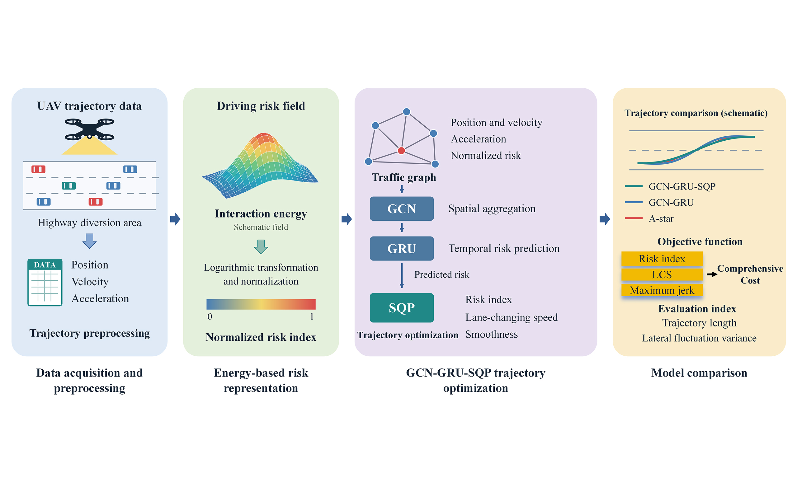
Highway diversion areas are critical traffic bottlenecks characterized by intensive interactions among vehicles. Conventional trajectory planning methods often struggle to capture the complex non-Euclidean spatial dependencies in these areas. This study presents a lane-changing trajectory optimization framework that integrates driving risk field theory with graph neural networks. Vehicle trajectories extracted from unmanned aerial vehicle videos are used to construct a spatial traffic graph incorporating normalized vehicle risk indices. A hybrid graph convolutional network-gated recurrent unit (GCN-GRU) module captures spatial interaction patterns and the temporal evolution of driving risk. Its risk predictions inform a sequential quadratic programming (SQP) objective that balances driving risk, lane-changing efficiency, and trajectory smoothness. In comparative experiments, the proposed GCN-GRU-SQP framework achieves a mean risk index of 0.15, a mean lane-changing speed of 18.35 m/s, a peak jerk of 1.5 m/s3, and a lateral fluctuation variance of 0.15. Its overall performance exceeds that of the GCN-GRU ablation baseline and the A-star algorithm. These findings support trajectory planning for mandatory lane changes in highway diversion areas.
Keywords


 Download PDF
1. INTRODUCTION
Frequent and unpredictable lane-changing maneuvers contribute to a higher incidence of collisions in highway diversion areas than on typical highway segments[1,2]. Accurate risk prediction and effective trajectory optimization can help improve traffic safety in these areas.
Conventional planning methods include graph search, sampling, and numerical optimization[3]. Search methods such as A-star identify feasible routes on a discretized representation, with resolution affecting both computational cost and path detail. Sampling-based methods explore continuous spaces; RRT* provides asymptotic optimality, although this does not guarantee an optimal solution within a finite planning budget[4]. For road vehicles, Werling et al. generated candidate trajectories in a Frenet frame and evaluated longitudinal and lateral motion costs[5]. Optimization-based planners can express motion constraints and competing objectives explicitly, but nonlinear formulations require suitable initialization and objective design[3]. These methods provide useful planning foundations; their application to interacting traffic also depends on how surrounding vehicles are represented.
Interaction-aware planning considers the dependence between an ego vehicle’s actions and the behavior of other road users. Schwarting et al. reviewed planning and decision-making under such interactions and uncertainty[6]. Zhang et al. combined learning-based cooperative decision-making with receding-horizon control for multiple autonomous vehicles at unsignalized intersections[7]. These studies support coordinated planning, while highway diversion areas introduce a different setting involving mandatory lane changes, adjacent-lane gaps, and motion toward the exit.
Graph-based temporal models offer a way to represent spatial dependencies that change over time. Temporal graph convolutional network (T-GCN) combines graph convolution with gated recurrent units (GRUs) for traffic prediction[8]. Extending data-driven graph modeling to multimodal transportation, Zhang et al. proposed Mixture of Spatial-Temporal Graph Transformer Networks, integrating a pattern-aware dynamic graph neural network, spatial-temporal graph transformers, and a mixture-of-experts framework to capture dependencies within and between taxi and shared bicycle data for urban congestion prediction[9]. At the agent level, Trajectron++ uses a graph-structured recurrent model to generate multimodal forecasts that account for heterogeneous agents and vehicle dynamics, with predictions that can be conditioned on an ego plan[10]. Complementing these graph-based representations, field-based models describe environmental influences and relative vehicle motion. Zong et al. combined molecular dynamics and field theory to represent static and dynamic elements at signalized intersections and support automated-vehicle trajectory planning[11]. At the traffic-flow level, Zong et al. proposed a traffic disorder model incorporating disturbance superposition and inter-vehicle kinematic discrepancies for congestion evolution analysis and prediction[12]. Together, these studies motivate combining spatiotemporal interaction modeling with explicit representations of environmental influences and relative motion; the present study applies this perspective to risk-aware lane-changing optimization in highway diversion areas. Such representations provide a basis for planning, but do not by themselves specify its trajectory objectives or constraints.
Recent work has more directly connected prediction with planning. Huang et al. integrated motion prediction with a differentiable nonlinear planner and learned its cost function through joint training[13]. Liang et al. developed an interaction-aware transformer predictor, pretrained it on human-driven trajectories, and transferred it using a limited dataset of interactions between autonomous and human-driven vehicles[14]. They further quantified prediction errors and incorporated the resulting uncertainty into motion planning. This study highlights the importance of both interaction modeling and the treatment of prediction errors when linking forecasts to planning. Together, these approaches motivate evaluating prediction through its role in trajectory generation, rather than relying only on forecasting accuracy.
Against this background, the present study examines how an energy-derived risk index can connect interaction representation, temporal risk prediction, and trajectory refinement in highway diversion areas. The graph convolutional network-gated recurrent unit (GCN-GRU) module predicts risk from a local traffic graph, and sequential quadratic programming (SQP) refines a candidate trajectory using risk, lane-changing speed (LCS), and smoothness objectives. The main contributions are summarized as follows.
(1) Risk representation: unmanned aerial vehicle (UAV) trajectories are used to compute energy-based interaction measures and convert them into normalized risk indices for highway diversion areas.
(2) Trajectory optimization: A GCN-GRU module models spatial interactions and temporal risk evolution. SQP uses the predicted risk to refine candidate trajectories under weighted risk, LCS, and smoothness objectives.
(3) Comparative evaluation: GCN-GRU-SQP is compared with GCN-GRU and A-star using the three objective components, trajectory length, and lateral fluctuation.
2. DRIVING ENERGY FIELD MODEL AND RISK METRICS
2.1. Driving energy field model
Artificial potential fields were introduced for real-time obstacle avoidance in manipulators and mobile robots[15]. Wolf and Burdick adapted potential functions to highway driving by representing lane, road, obstacle, and speed-related effects[16]. Wang et al. formulated a driving risk field based on driver–vehicle–road interactions[17]. Subsequent work applied driving safety fields to pre-collision warning[18] and risk potential fields to multi-vehicle interactions in weaving areas[19]. Building on these formulations, this study represents surrounding vehicles and the exit ramp as energy sources and evaluates their combined influence during diversion-area lane changes.
Following the field-based interaction models of Wang et al.[18] and Ma et al.[19], the vehicle and ramp contributions are expressed by:
where Md is the equivalent mass of the energy source. θr is the angle between speed direction and energy source. ω = L, if the energy source is the ramp, ω = av, if the energy source is a vehicle. r is the distance from the vehicle to discrete energy source. According to our recent research, c = 1 for surrounding vehicles, c = -1 for exit ramp[20].
According to the electromagnetic field theory and artificial potential field theory, the influence of surrounding vehicles on a specific vehicle can be calculated as:
Δd is the proportion of spatial movement of ego-vehicle relative to the ramp or surrounding vehicle per unit time.
The field energy of the ego vehicle is equal to the work done by the combined forces in:
where α1 = 0.29, α2 = 2.00, α3 = -0.89, which are obtained through training with real-world scenario data and genetic algorithms. Therefore, the energy value of the ego vehicle is determined by the combined influence of surrounding vehicles[18].
The energy field model serves as a core component that quantifies vehicle interaction risks into interpretable energy values, which are key input features for graph convolutional network (GCN) and embedded into the loss function to constrain high-risk behaviors. It unifies risk quantification, feature representation, and behavior guidance throughout the framework.
2.2. Dataset
This study captured a series of full-area videos of the diversion area on Shanghai Middle Ring Expressway using an UAV. In this scenario, frequent lane-changing behavior reduces traffic efficiency and safety. Vehicle trajectory data were extracted by integrating high-precision orthophoto maps with the You Only Look Once version 5 (YOLOv5) algorithm. First, the orthophoto maps were used to calibrate the UAV video imagery to geographic coordinates, establishing an accurate alignment between real-world road locations and video pixel positions. The YOLOv5 algorithm was then applied to perform real-time detection and tracking of all vehicles in the UAV video frames. Leveraging the calibrated geographic coordinate system, the vehicle ID, frame number, lane information, and X/Y geographic coordinates were extracted for each vehicle in every frame. The results are shown in Figure 1. The UAV video screenshots in Figure 1 show vehicles from an overhead viewpoint. No identifiable faces or license-plate information are visible in the images; therefore, the images presented in this study do not disclose personally identifiable information.
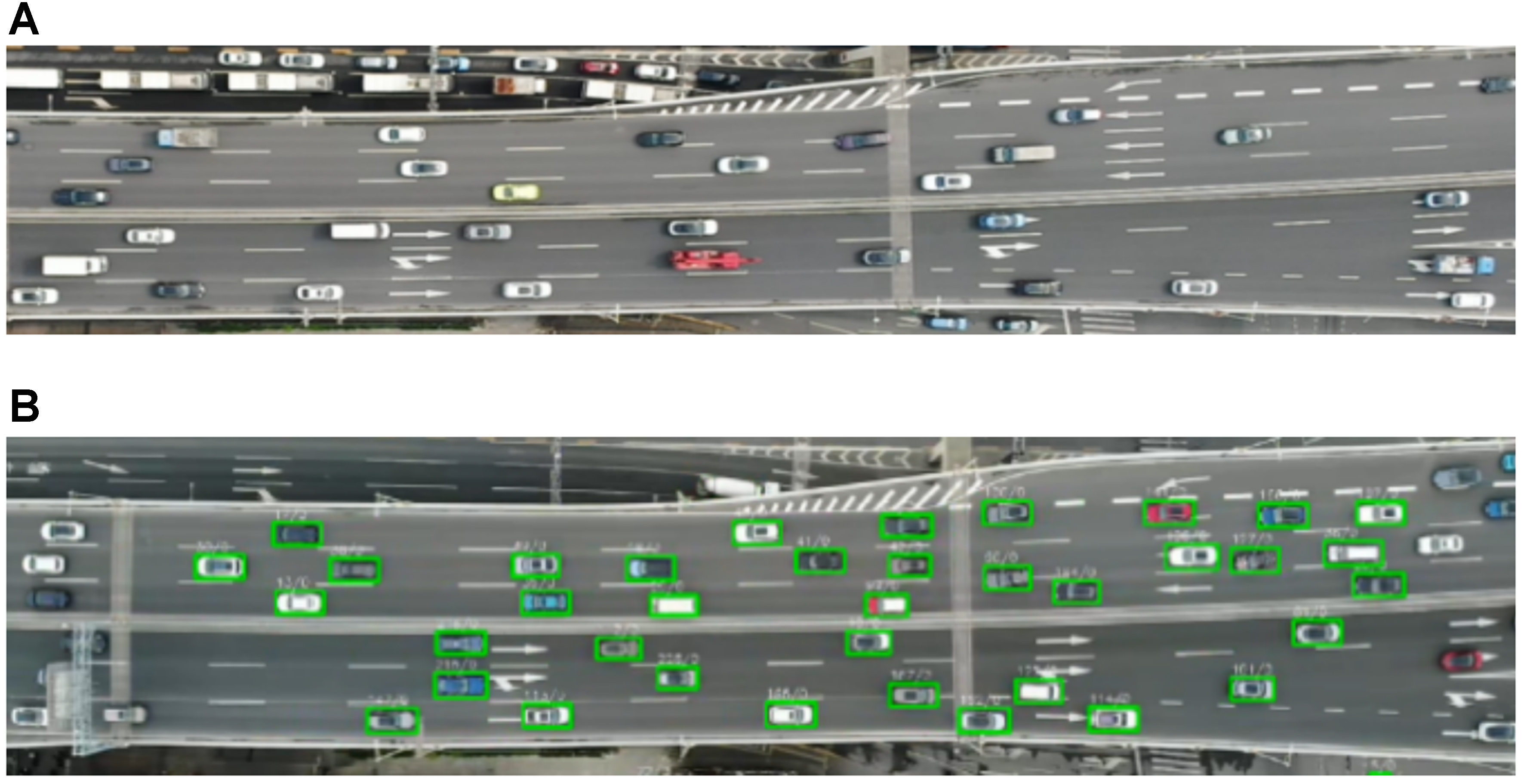
Figure 1. Diversion area of Shanghai Middle Ring expressway. (A) High-precision orthophoto maps; (B) Vehicle detection and trajectory data based on YOLOv5. Photographed by the authors. YOLOv5: You Only Look Once version 5.
The raw data included the number of frames, Car IDs, X-coordinates, Y-coordinates, and the lane number of all vehicles in each frame (as shown in Table 1, vehicle recognition accuracy: 100%). A total of 1,794 valid lane-changing event samples were finally retained after data screening. Based on the orthophoto base map, the vehicle position recognition accuracy reaches 0.02 m, meeting the lane-level recognition precision requirement (deviation rate: 0.57%).
Data explanation
| Variable name | Explanation |
| Frame NUM | Number of frames (30 frames per second) |
| Car ID | Vehicle ID |
| X-coordinate | Driving direction of the vehicle |
| Y-coordinate | The road cross-section |
| Lane | Lane where the vehicle is located |
The raw data is preprocessed to derive key kinematic parameters, including vehicle speed, acceleration, relative distance, and orientation angle. Subsequently, the interaction forces and field intensities are calculated using Equations (1)-(4), from which the field energy of the ego vehicle is determined via Equation (5). Defined as the cumulative work done by the combined interaction forces from surrounding traffic and road constraints, this energy value serves as a core quantitative metric that translates complex multi-vehicle conflicts into interpretable driving risks. To visualize the spatial distribution of these risks, Figure 2 visualizes the energy-field evolution on a single representative left-direction lane-change event sampled from the dataset; it is used only to illustrate the before/during/after energy pattern. In these maps, the X-axis represents the vehicle’s driving direction, the Y-axis denotes the road cross-section, and the Z-axis corresponds to the quantified vehicle energy value.
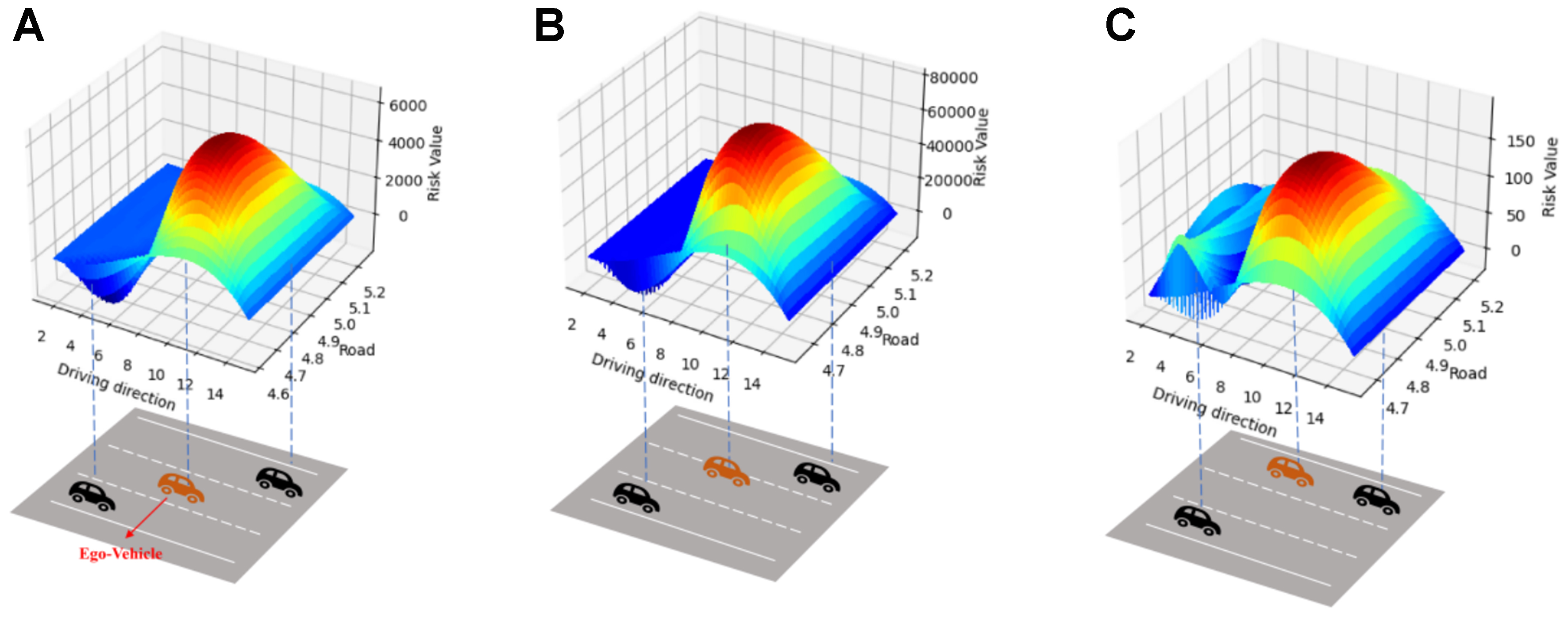
Figure 2. Heat maps of entire vehicle lane-changing behavior. (A) Before lane-changing behavior; (B) During lane-changing process; (C) After lane-changing behavior.
• Before the lane-changing behavior, the energy value around the ego vehicle is relatively high. Therefore, it will move towards the direction of lower energy value, which means it will change to the left lane in the next moment.
• During the lane-changing process, the energy value of the ego vehicle reaches its peak, indicating maximum vehicle interaction intensity and the highest energy level in the lane-changing process.
• After the lane-changing behavior is completed, the energy values of all vehicles in this section decrease gradually to an acceptable state.
The energy value in Equation (5) quantifies vehicle interactions. Under the assumption that higher energy indicates stronger interaction risk, it is converted into a relative risk index for prediction and trajectory optimization. Logarithmic transformation reduces the influence of extreme values, while normalization produces a dimensionless feature that can be balanced with efficiency and smoothness. The transformation is defined as
where qi,t is the shifted dimensionless energy score; Emin and Emax are the training-set energy extrema; Es > 0 is a fixed energy scale; and qmax is the maximum training score. Ri,t is the normalized risk index. ln denotes the natural logarithm, and clip (0,1) limits its argument to [0,1]. The same normalization parameters are used for validation and prediction.
3. LANE CHANGING TRAJECTORY OPTIMIZATION
3.1. Optimization framework
In this study, a GCN-GRU-SQP framework is developed for lane-changing trajectory optimization within highway diversion zones. As depicted in Figure 3, vehicle attributes are initially structured into a traffic graph representation. GCNs are adopted to aggregate information of neighboring vehicles and extract spatial interaction features. GRUs are then utilized to model the temporal evolution of spatial features and perform next-step risk prediction. At the final stage, SQP optimizes and refines candidate trajectories with respect to three metrics: risk index, LCS, and trajectory smoothness, which jointly constitute the comprehensive cost.
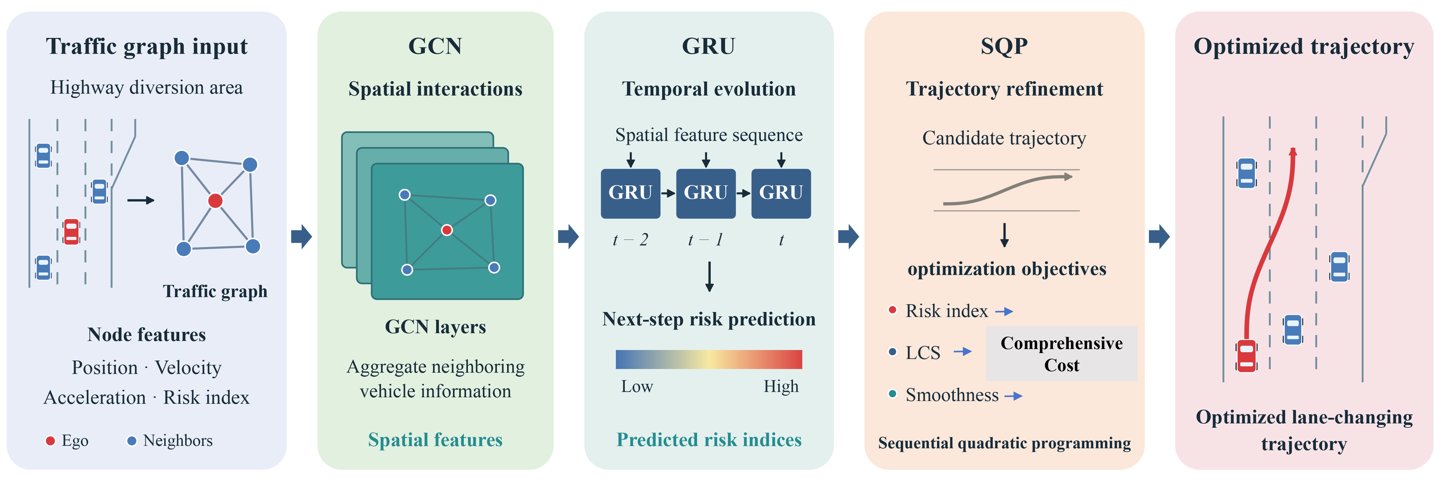
Figure 3. GCN-GRU-SQP trajectory optimization model structure. GCN-GRU-SQP: Graph convolutional network-gated recurrent unit-sequential quadratic programming; LCS: lane-changing speed.
Vehicles are defined as graph nodes, with edges connecting vehicles within 30 m. This threshold is derived from real driving conditions. At highway diversion sections, vehicle speeds are 15-25 m/s (54-90 km/h), and drivers mainly consider surrounding vehicles within a 2-second preview window (roughly 30-50 m) for lane-change decisions. Vehicles in the target lane within 30 m directly determine the feasibility of ego-vehicle lane change, whereas vehicles farther than 30 m exhibit little relative position change during the lane-change maneuver and impose trivial influences. The 30 m threshold is thereby selected for graph construction to capture critical traffic interactions and avoid redundant noise from distant vehicles. Each node contains six features: longitudinal and lateral position, the two velocity components, longitudinal acceleration, and normalized risk. These constitute the input matrix fed into the GCN, and its spatial aggregation operation follows the formulation proposed by Kipf and Welling[21].
where At is the adjacency matrix, I is the identity matrix, and Dt is the diagonal degree matrix of At+I. Ht(l) denotes the features at layer l, initialized by Xt; W(l) and b(l) are trainable weights and biases, and ReLU is the rectified linear activation.
The resulting node embedding zi,t is passed to GRU in chronological order. The hidden state and next-step risk are obtained as[22]
where hi,t is the temporal hidden state, wo and bo are the output weights and bias, and σ is the sigmoid function. The superscript T denotes transpose, and
For a selected target-lane gap, feasible candidate trajectories are first generated using quintic lateral curves[5]. GCN-GRU predicts the interaction risk associated with each candidate rather than directly outputting trajectory coordinates. Whenever SQP updates the candidate states, the corresponding graph features and connections are reconstructed, and the energy-derived risk inputs are recalculated using the formulation in Section 2. The same trained GCN-GRU, with its parameters fixed, is then evaluated again to obtain updated candidate-dependent risk predictions. Thus, the risk term varies with the candidate trajectory throughout optimization. SQP jointly considers this updated risk, LCS, and trajectory smoothness through the following three objective components:
JR, JLCS, and Jsmooth represent mean risk, mean longitudinal speed, and peak jerk. k indexes the K planning steps;
where J is the combined cost, vmax is the speed limit, and jmax is the jerk limit. The weights for risk, LCS, and smoothness are set to 0.50, 0.25, and 0.25, respectively. This safety-oriented choice is motivated by frequent vehicle interactions and restricted maneuvering space in highway diversion areas. Gao et al. reported that, under high-density conditions with frequent interactions and short headways, the safety weight in risk-field-based trajectory optimization should be increased to 0.40-0.50 to preserve safety margins, accepting a modest reduction in efficiency[23]. This finding supports assigning risk a higher weight than either LCS or smoothness in the present study, although their four-objective formulation differs from ours. Here, the two secondary objectives receive equal weights to retain both speed and ride comfort. For feasible trajectories satisfying the stated speed and jerk bounds, the three component costs in Equation (13) lie in [0,1], making their weights comparable on a dimensionless scale. The 0.50:0.25:0.25 ratio is a design choice for this study, rather than a universally optimal ratio established by the cited work. The larger risk coefficient gives risk twice the marginal penalty of either secondary cost for equal normalized changes; it does not impose an absolute safety priority or guarantee collision avoidance.
SQP solves the objective through local quadratic approximations[24], subject to road boundaries, longitudinal speed between zero and vmax, and acceleration and jerk limits. Maximum jerk is handled through an auxiliary upper bound constrained to exceed the jerk magnitude at each planning step. The risk term penalizes interaction intensity; it does not by itself guarantee collision avoidance. The first feasible optimized segment is retained, and planning repeats as new observations arrive. Table 2 lists the planner parameters.
Trajectory planner parameters
| Parameter | Value | Parameter | Value |
| The sampling interval | Δt = 1/30 s | Lane displacement | 3.5 m |
| Test-section longitudinal length | 20 m | Interaction radius | 30 m |
| Risk weight | 0.50 | Maximum jerk | 3.0 m/s3 |
| Acceleration bounds | [-3.0,2.0] m/s2 | SQP iterations | 30 |
| Risk horizon | 15 frames | Tolerance | 10-3 |
| LCS weight | 0.25 | Smoothness weight | 0.25 |
| Speed limit | 25 m/s |
3.2. Model training
The dataset contains 1,794 lane-changing events. A 6:2:2 training protocol is used, corresponding to 1,076 training events, 359 validation events, and 359 prediction (test) events. Frames from the same event remain in one subset to prevent data leakage across sets. Adam updates the network parameters using the training set only. The single checkpoint with the lowest validation loss is selected for final evaluation. At the end of each epoch, the test set is evaluated once by forward computation without backpropagation, solely to plot the test-loss curve in Figure 4. Test results are not used for gradient updates, best-epoch selection, early stopping, or any hyperparameter tuning. Table 3 summarizes the training settings.
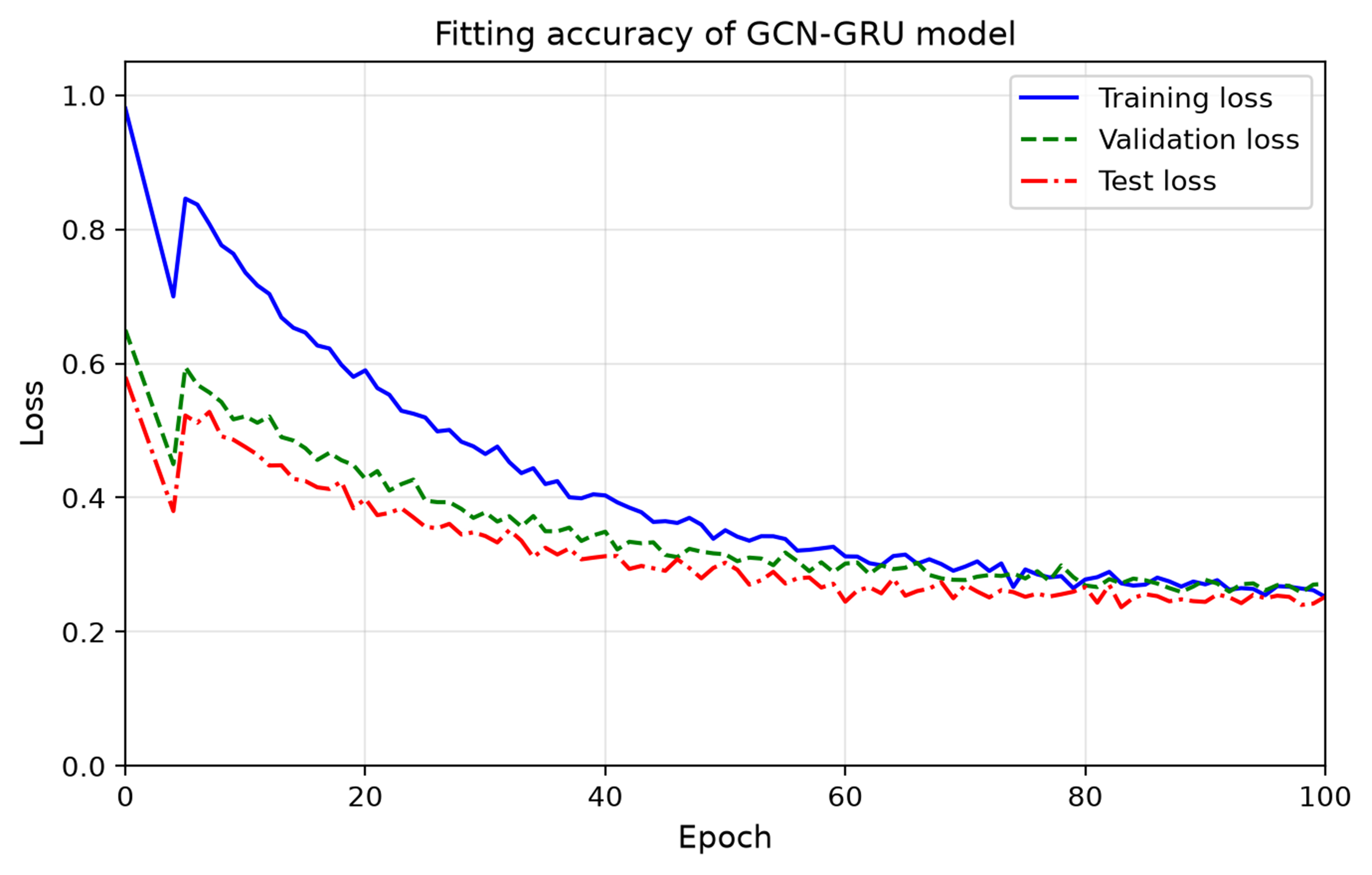
Figure 4. Loss curves of the GCN-GRU model. GCN-GRU: Graph convolutional network-gated recurrent unit.
Model structure and parameters
| Parameter | Value | Parameter | Value |
| GCN layers | 2 | Activation function | ReLU |
| GRU hidden units | 64 | GRU layers | 1 |
| Optimizer | Adam | Learning rate | 0.001 |
| Epochs | 100 | Batch size | 32 |
| Dropout | 0.2 | Random seed | 42 |
| Train/validation/prediction | 60%/20%/20% | Prediction horizon | 15 frames |
| GPU | RTX 3060 | Framework | PyTorch 2.0 |
The GCN-GRU is trained using the mean squared error between predicted and observed risk indices:
where Lpred is the prediction loss, n indexes the M valid targets, and
Model comparison results
| Evaluation indicators | Optimization model | |||
| GCN-GRU-SQP | GCN-GRU | A-star | ||
| Efficiency indicators | JLCS (m/s) | 18.35 | 10.62 | 10.58 |
| Safety indicators | JR | 0.15 | 0.08 | 0.38 |
| Smoothness Indicators | Jsmooth (m/s3) | 1.5 | 2.5 | 3.0 |
| Comprehensive cost (minξJ) | 0.27 | 0.39 | 0.58 | |
3.3. Model comparison
To comprehensively verify the overall performance of the proposed GCN-GRU-SQP framework for lane-changing trajectory optimization in highway diversion areas, the GCN-GRU risk-prediction-only baseline and the classic A-star search-based planner are adopted for comparative evaluation from safety, lane-changing efficiency and trajectory smoothness perspectives, as summarized in Table 4. The quantitative results reveal that the proposed GCN-GRU-SQP framework obtains superior comprehensive cost performance over the two comparison methods.
From the safety perspective, the GCN-GRU baseline achieves the lowest mean risk index of 0.08, as it focuses purely on risk prediction and tends to produce overly conservative motion solutions to pursue minimal interaction risk. Nevertheless, the GCN-GRU-SQP model still maintains a satisfactorily low risk index of 0.15, keeping vehicle-to-vehicle interaction at a mild level during lane-change maneuvers. By contrast, the A-star algorithm yields the highest risk value of 0.38, because traditional graph-search planning lacks explicit modeling of dynamic multi-vehicle interaction risks. In terms of lane-changing efficiency, the proposed framework realizes an average LCS of 18.35 m/s, substantially exceeding the performance of GCN-GRU (10.62 m/s) and A-star (10.58 m/s). It illustrates that the SQP optimizer can adequately exploit valid gaps in target lanes under the constraint of predicted risk indices. Different from the over-conservative tendency of pure risk-prediction outputs, SQP makes reasonable trade-offs between safety and driving efficiency. Regarding trajectory smoothness, the GCN-GRU-SQP approach yields a peak jerk of only 1.5 m/s3, lower than 2.5 m/s3 for GCN-GRU and 3.0 m/s3 for A-star. The step-wise discrete path generated by the A-star algorithm introduces frequent steering inflection points and severe lateral oscillation; even though GCN-GRU outputs continuous trajectories, it cannot further optimize motion smoothness. Benefiting from numerical optimization, GCN-GRU-SQP effectively suppresses abrupt motion variation and improves ride comfort. Overall, the GCN-GRU-SQP framework achieves the minimal comprehensive weighted cost of 0.27, which proves that embedding spatio-temporal risk prediction into the numerical optimization loop can well balance safety, efficiency and smoothness requirements for autonomous lane-changing in complex diversion-area traffic scenarios.
Beyond the aforementioned objective-function-related evaluation metrics, further macroscopic geometric indicators, namely lane-changing trajectory length and lateral fluctuation variance, are analyzed in Figure 5 and Table 5. The test scenario is a 20-m-long highway diversion segment, in which the ego vehicle performs a left-direction lane-change to avoid vehicles heading for the off-ramp. Figure 5 plots the averaged lane-changing trajectories from 40 vehicle samples on a two-lane road with 3.5 m lane width.
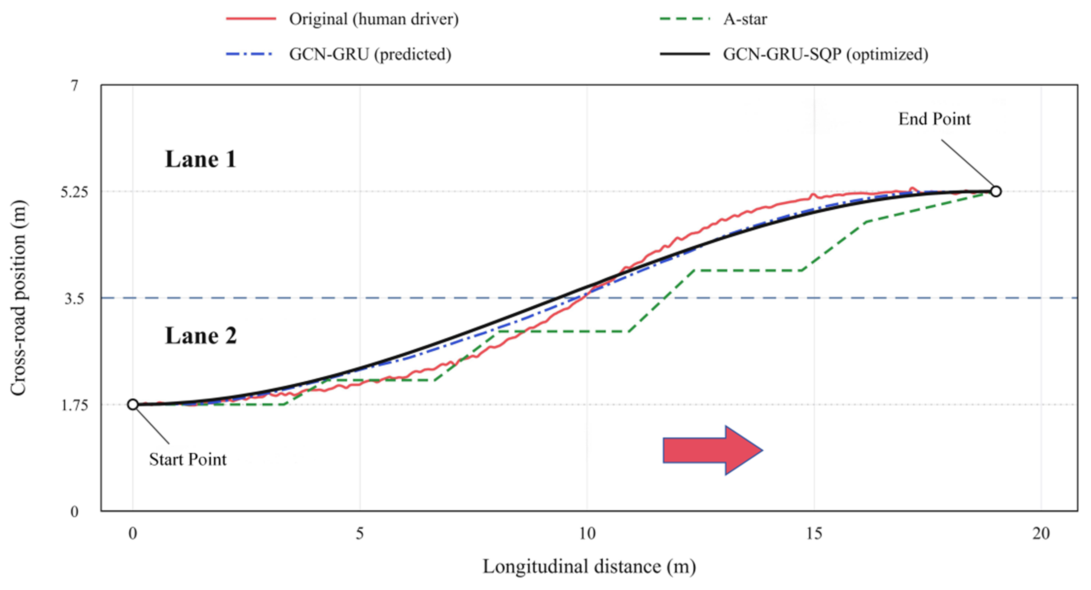
Figure 5. Trajectory optimization comparison. GCN-GRU-SQP: Graph convolutional network-gated recurrent unit-sequential quadratic programming.
Lane-changing trajectory comparison
| Model | Lane-changing trajectory length (m) | Lane-changing trajectory lateral fluctuation variance (m2) |
| Original data | 22.6 | 1.28 |
| A-star algorithm | 22.0 | 0.95 |
| GCN-GRU | 19.8 | 0.32 |
| GCN-GRU-SQP | 19.7 | 0.15 |
The original human-driven trajectory presents a tortuous shape with considerable path redundancy, achieving a trajectory length of 22.6 m and a lateral fluctuation variance of 1.28. The A-star algorithm reduces the trajectory length to 22.0 m and lateral variance to 0.95, yet the optimization improvement is marginal. In addition, its output contains step-wise path segments and frequent steering inflection points, failing to generate continuous smooth lane-changing motions. Both GCN-GRU and GCN-GRU-SQP produce continuous smooth trajectories with markedly shortened path length and mitigated lateral fluctuations. The GCN-GRU prediction-only model yields a trajectory length of 19.8 m and a lateral fluctuation variance of 0.32. As the optimal solution among all competitors, GCN-GRU-SQP obtains the minimal trajectory length of 19.7 m and the lowest lateral fluctuation variance of 0.15, demonstrating superior trajectory linearity and lateral stability. Compared with the traditional search-based algorithm and pure prediction baseline, the proposed GCN-GRU-SQP framework shortens lane-change travel distance and suppresses lateral oscillations, and effectively balances lane-changing efficiency, safety and driving comfort.
Table 5 reports the lateral deviation variance σlat2 in m2, computed over the whole manoeuvre about the lane reference:
where yi is the lateral position and
which excludes the lane-change displacement and equals 2.99 × 10⁻⁶ m at zero noise. Both are aggregated over the N points of a single complete trajectory without averaging across samples. The two are not the same indicator and are not interchangeable. The 0.15 m2 in Table 5 is σlat2 measured about the lane reference, which retains the ~3.5 m lane-change displacement, whereas the zero-noise baseline is εlat measured about the smoothed reference with that component removed. Because the references differ, √0.15 m2 does not give 2.99 × 10⁻⁶ m; the two are not interconvertible, and no comparison is drawn between them.
3.4. Sensitivity analysis
A sensitivity analysis distinguishes two error sources. For the trajectory-point error, the observed noise of 0.0955 m, about five times the 0.02 m accuracy in Section 2.2, is the operating point, with the four lengths (22.6, 22.0, 19.8, 19.7 m) and the jerk ordering of Table 4 as baselines. Only GCN-GRU-SQP is perturbed, A-star and GCN-GRU being fixed references. For the risk-value error, the P50 and P90 cut-points of 0.2098 and 0.3335 divide the 1,794 samples into low, moderate and high classes at 50.00%, 39.97% and 10.03%.
Figure 6 analyzes position noise. The jerk baseline here uses a shorter smoothing window than Table 4, since this section examines the response to injected noise rather than reporting the smoothed performance value. The same trajectory therefore yields 3.12 m/s3 here and 1.5 m/s3 in Table 4, while the ordering among the three schemes is unaffected. Jerk follows the definition of Equation (12), with the sampling interval Δt = 1/30 s ≈ 0.0333 s given by the 30 Hz frame rate in Table 1. For Table 4 the position series is smoothed with a Savitzky-Golay filter, window = 9 frames, order = 3, before differentiation, whereas for Figure 6C no additional smoothing beyond the minimal differentiation is applied. The processing pipeline proceeds from the raw position series, through optional smoothing and numerical differentiation to acceleration, then to jerk per Equation (12), and finally to the maximum over the trajectory. Position noise is injected at the input stage by adding a zero-mean Gaussian perturbation of standard deviation σ to each sampled coordinate, after which velocity, acceleration and jerk are re-derived by numerical differentiation. Figure 6A length is stable. It is 19.700 m without noise and 20.489 m at σ = 0.50 m, a 4.01% deviation. It stays shorter than the 22.000 m A-star baseline. Efficiency holds. Figure 6B lateral fluctuation is sensitive. It rises from 2.99 × 10⁻⁶ to 1.89 ×
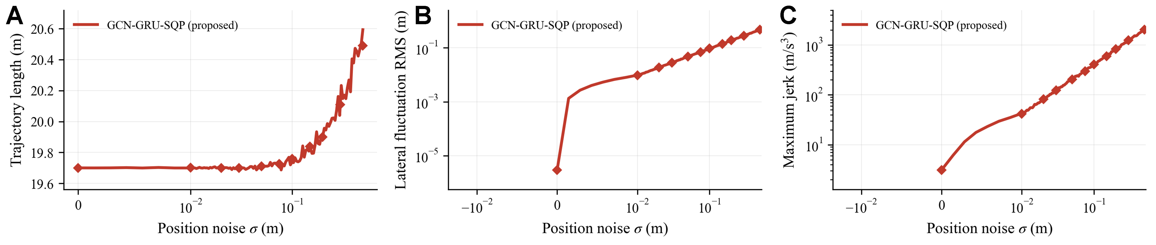
Figure 6. Trajectory-point sensitivity analysis of the proposed GCN-GRU-SQP. (A) Trajectory length; (B) Lateral fluctuation RMS; (C) Maximum jerk. GCN-GRU-SQP: Graph convolutional network-gated recurrent unit-sequential quadratic programming; RMS: root mean square.
Figure 7 analyzes risk perturbation. Figure 7A class composition shifts. High-risk share is 10.03% at baseline and moves to 21.74% and 4.74% under δ = ±20%. Figure 7B fixed cut-points yield 12.4% reclassification at δ = ±10%. Recalibrated cut-points yield 0% at any δ. Relative ranking is immune to multiplicative bias. Fixed-cut sensitivity measures cross-dataset transfer error. Figure 7C normalization bound matters. Raw extremes differ by eight orders. Mean normalized risk is 0.217 at P99.5 cap and 0.510 at P95 cap. Winsorizing removes extreme dominance.
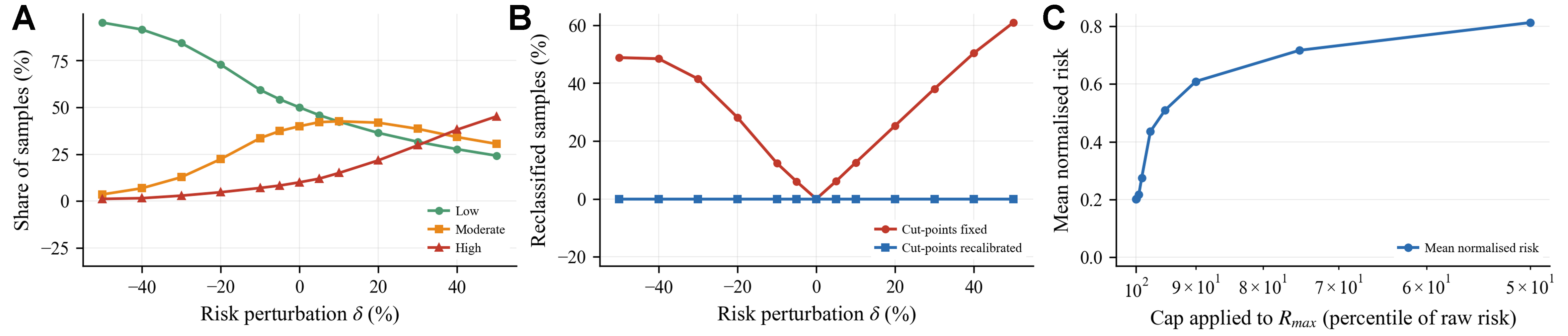
Figure 7. Risk-value sensitivity analysis. (A) Risk-class composition; (B) Reclassification rate; (C) Normalisation bound.
Figure 8 compares both errors. Figure 8A trajectory-point index saturates near 50 early due to capped smoothness criteria. Risk-value index rises gradually. At measured noise (2.73% lane width), trajectory-point error dominates. Perception is binding. Figure 8B critical perturbation ranks clearly. Jerk doubles at 0.023% and fluctuation degrades at 0.183% first. Five percent reclassification occurs at 4.12% and high-risk shift occurs at 4.98% later. Length changes by 1% at 5.638%. Trajectory-point error is the bottleneck. It does not overturn the robust findings on path length and scheme ordering.
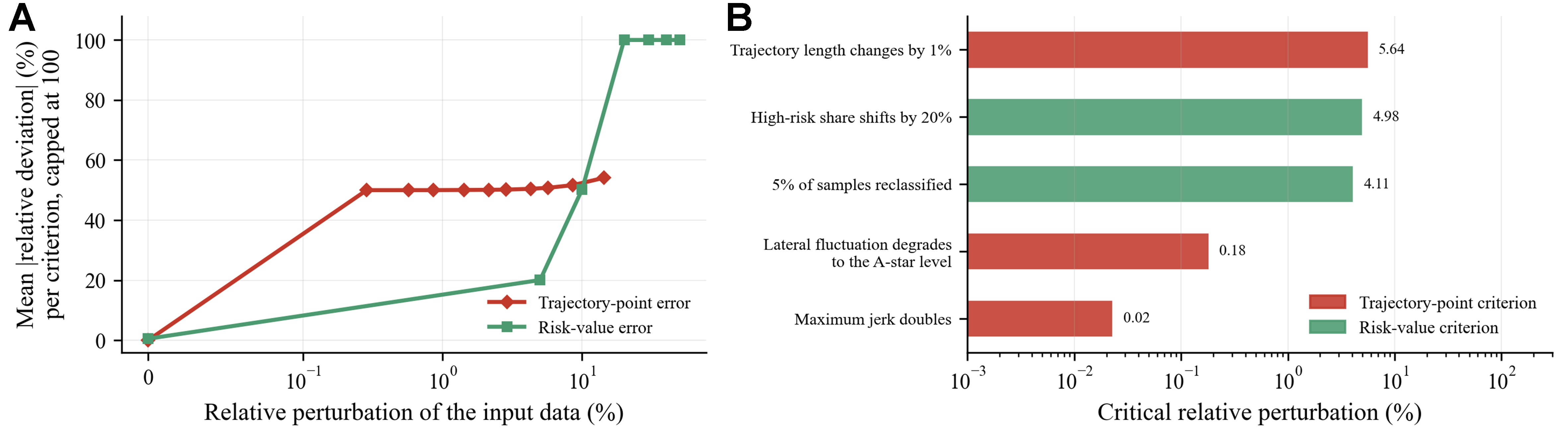
Figure 8. Quantitative comparison of the two error sources. (A) Composite destabilisation index; (B) Critical perturbation level.
4. CONCLUSIONS
This study develops a vehicle-level risk metric based on driving risk field theory and UAV-derived trajectories to connect vehicle interactions with the spatial structure of traffic. The proposed GCN-GRU-SQP framework uses this metric for lane-changing trajectory optimization. The GCN-GRU captures non-Euclidean spatial interactions and the temporal evolution of risk, and its predictions inform the SQP objective. SQP then refines candidate trajectories by balancing risk, lane-changing efficiency, and motion smoothness. In the evaluated scenarios, GCN-GRU-SQP achieves a lower combined cost than the GCN-GRU baseline and A-star. It produces a mean LCS of 18.35 m/s, a mean risk index of 0.15, a peak jerk of
The sensitivity analysis clarifies the framework’s applicability. Trajectory length is relatively robust to estimation errors, whereas smoothness metrics are highly sensitive to positioning accuracy and smoothing settings. Relative risk rankings remain stable under multiplicative bias, indicating that threshold sensitivity is primarily associated with transfer between datasets and the choice of normalization bounds. Trajectory-point errors affect smoothness before substantially changing path length or the relative performance of the methods, identifying perception accuracy as a key limitation.
The study has several limitations. Evaluation is restricted to UAV data from a single diversion area, and the dataset lacks detailed vehicle dynamics measurements, including steering and tire–road adhesion information. The proposed approach is therefore a traffic-level planning tool and is not yet suitable for direct deployment in autonomous vehicles. Future work will incorporate data from multiple scenarios and more complete vehicle dynamics constraints to support real-time cooperative control of connected automated vehicles.
DECLARATIONS
Authors’ contributions
Conceptualization, methodology, supervision, writing - review and editing: Li, Y.
Data curation, formal analysis, writing - original draft: Wu, Y.
Supervision, investigation: Chen, X.
All authors reviewed the results and approved the final version of the manuscript.
Availability of data and materials
The original contributions presented in this study are included in the article. Further inquiries can be directed to the corresponding author.
AI and AI-assisted tools statement
During the preparation of this manuscript, the AI tool Gemini 3.1 Pro (Google, released February 2024) was used solely for language editing. The tool did not influence the study design, data collection, analysis, interpretation, or the scientific content of the work. All authors take full responsibility for the accuracy, integrity, and final content of the manuscript.
Financial support and sponsorship
This research was supported by the National Natural Science Foundation of China (Grant Nos. 52202419 and 52472347) and the Open Fund of State Key Laboratory of Maritime Technology and Safety.
Conflicts of interest
Chen, X. serves as a Section Member of the Multimodal Perception and Computer Vision section. Chen, X. is affiliated with Shanghai Ship and Shipping Research Institute Co., Ltd., but was not involved in any steps of editorial processing, notably including reviewer selection, manuscript handling, and decision-making, while the other authors have declared that they have no conflicts of interest.
Ethical approval and consent to participate
Not applicable.
Consent for publication
Not applicable.
Copyright
© The Author(s) 2026.
REFERENCES
1. Xu, T.; Zhang, Z.; Wu, X.; Qi, L.; Han, Y. Recognition of lane-changing behaviour with machine learning methods at freeway off-ramps. Physica. A. 2021, 567, 125691.
2. Du, W. J.; Xia, G. D.; Chen, F.; Pan, X. D. Research on safety of freeway off-ramp lane changing behavior based on lateral force coefficient. In Access Management Theories and Practices, Shanghai, China. 2015; pp. 201-10.
3. Paden, B.; Cap, M.; Yong, S. Z.; Yershov, D.; Frazzoli, E. A survey of motion planning and control techniques for self-driving urban vehicles. IEEE. Trans. Intell. Veh. 2016, 1, 33-55.
4. Karaman, S.; Frazzoli, E. Sampling-based algorithms for optimal motion planning. Int. J. Robot. Res. 2011, 30, 846-94.
5. Werling, M.; Ziegler, J.; Kammel, S.; Thrun, S. Optimal trajectory generation for dynamic street scenarios in a Frenét Frame. In Proceedings of the 2010 IEEE International Conference on Robotics and Automation, Anchorage, USA. May 03-07, 2010. IEEE; 2010. pp. 987-93.
6. Schwarting, W.; Alonso-Mora, J.; Rus, D. Planning and decision-making for autonomous vehicles. Annu. Rev. Control. Robot. Auton. Syst. 2018, 1, 187-210.
7. Zhang, R.; Xu, X.; Lu, Y.; Xu, X.; Zhang, X.; Ma, Q. Learning-based cooperative decision-making and control for multiple autonomous vehicles in unsignalized intersections. Intell. Robot. 2025, 5, 695-716.
8. Zhao, L.; Song, Y.; Zhang, C.; et al. T-GCN: a temporal graph convolutional network for traffic prediction. IEEE. Trans. Intell. Transport. Syst. 2020, 21, 3848-58.
9. Zhang, J.; Chen, Y.; Wang, T.; Xie, C. T.; Tian, Y. Mixture of Spatial–Temporal Graph Transformer Networks for urban congestion prediction using multimodal transportation data. Expert. Syst. Appl. 2025, 268, 126108.
10. Salzmann, T.; Ivanovic, B.; Chakravarty, P.; Pavone, M. Trajectron++: dynamically-feasible trajectory forecasting with heterogeneous data. In Computer Vision - ECCV 2020. Cham: Springer International Publishing; 2020. pp. 683-700.
11. Zong, F.; Yue, S.; Zeng, M.; Liu, Y.; Tang, J. Environment reconstruction and trajectory planning for automated vehicles driving through signal intersection. Physica. A. 2025, 660, 130323.
12. Zong, F.; Li, Y. X.; Zeng, M. A traffic disorder model for congestion evolution analysis and traffic flow prediction: considering disturbance superposition and inter-vehicle kinematic discrepancies. Expert. Syst. Appl. 2026, 330, 133023.
13. Huang, Z.; Liu, H.; Wu, J.; Lv, C. Differentiable integrated motion prediction and planning with learnable cost function for autonomous driving. IEEE. Trans. Neural. Netw. Learn. Syst. 2024, 35, 15222-36.
14. Liang, J.; Tan, C.; Yan, L.; Zhou, J.; Yin, G.; Yang, K. Interaction-aware trajectory prediction for safe motion planning in autonomous driving: a transformer-transfer learning approach. IEEE. Trans. Intell. Transport. Syst. 2025, 26, 17080-95.
15. Khatib, O. Real-time obstacle avoidance for manipulators and mobile robots. Int. J. Robot. Res. 1986, 5, 90-8.
16. Wolf, M. T.; Burdick, J. W. Artificial potential functions for highway driving with collision avoidance. In Proceedings of the 2008 IEEE International Conference on Robotics and Automation, Pasadena, USA. May 19-23, 2008. IEEE; 2008; pp. 3731-6.
17. Wang, J.; Wu, J.; Li, Y. Concept, principle and modeling of driving risk field based on driver-vehicle-road interaction. China. J. Highway. Transp. 2016, 29, 105-14.
18. Wang, J.; Wu, J.; Zheng, X.; Ni, D.; Li, K. Driving safety field theory modeling and its application in pre-collision warning system. Transp. Res. Part. C. Emerg. Technol. 2016, 72, 306-24.
19. Ma, Y.; Dong, F.; Yin, B.; Lou, Y. Real-time risk assessment model for multi-vehicle interaction of connected and autonomous vehicles in weaving area based on risk potential field. Physica. A. 2023, 620, 128725.
20. Li, Y.; Cai, J.; Chen, X.; Tang, S.; Wang, Z. A novel data-driven theory for interactive behavior and risk assessment modelling in urban expressway weaving sections: evidence from UAV data and transformer models. Transp. Res. Part. C. Emerg. Technol. 2026, 185, 105589.
21. Kipf, T. N.; Welling, M. Semi-supervised classification with graph convolutional networks. arXiv 2016, arXiv:1609.02907. Available online: https://doi.org/10.48550/arXiv.1609.02907. (accessed 2026-11-13).
22. Cho, K.; van Merriënboer, B.; Gulcehre, C.; et al. Learning phrase representations using RNN encoder-decoder for statistical machine translation. In Proceedings of the 2014 Conference on Empirical Methods in Natural Language Processing, Doha, Qatar. Association for Computational Linguistics; 2014. pp. 1724-34.
23. Gao, J.; Liu, W.; Liu, P.; Bai, P.; Xie, C. Multi-objective trajectory optimization for autonomous vehicles based on an improved driving risk field. Modelling 2026, 7, 75.
24. Kraft, D. A software package for sequential quadratic programming. Technical Report DFVLR-FB 88-28. 1988. https://degenerateconic.com/uploads/2018/03/DFVLR_FB_88_28.pdf. (accessed 2026-11-13).
Cite This Article
 Open Access
How to Cite
Li, Y.; Wu, Y.; Chen, X. From assessment to optimization: GCN for lane-changing trajectory planning in highway diversion area. Intell. Robot. 2026, 6(4), 970-84. https://dx.doi.org/10.20517/ir.2026.41
Download Citation
If you have the appropriate software installed, you can download article citation data to the citation manager of your choice. Simply select your manager software from the list below and click on download.
Export Citation File
Type of Import
Tips on Downloading Citation
Citation Manager File Format
Type of Import
Direct Import: When the Direct Import option is selected (the default state), a dialogue box will give you the option to Save or Open the downloaded citation data. Choosing Open will either launch your citation manager or give you a choice of applications with which to use the metadata. The Save option saves the file locally for later use.
Indirect Import: When the Indirect Import option is selected, the metadata is displayed and may be copied and pasted as needed.
About This Article
Special Topic
Copyright

Data & Comments
Data
0










Comments
Comments must be written in English. Spam, offensive content, impersonation, and private information will not be permitted. If any comment is reported and identified as inappropriate content by OAE staff, the comment will be removed without notice. If you have any queries or need any help, please contact us at [email protected].