



Measurement of silicon carbide epilayer thickness using physics-informed neural networks and hybrid intelligent systems
 0
0 Abstract
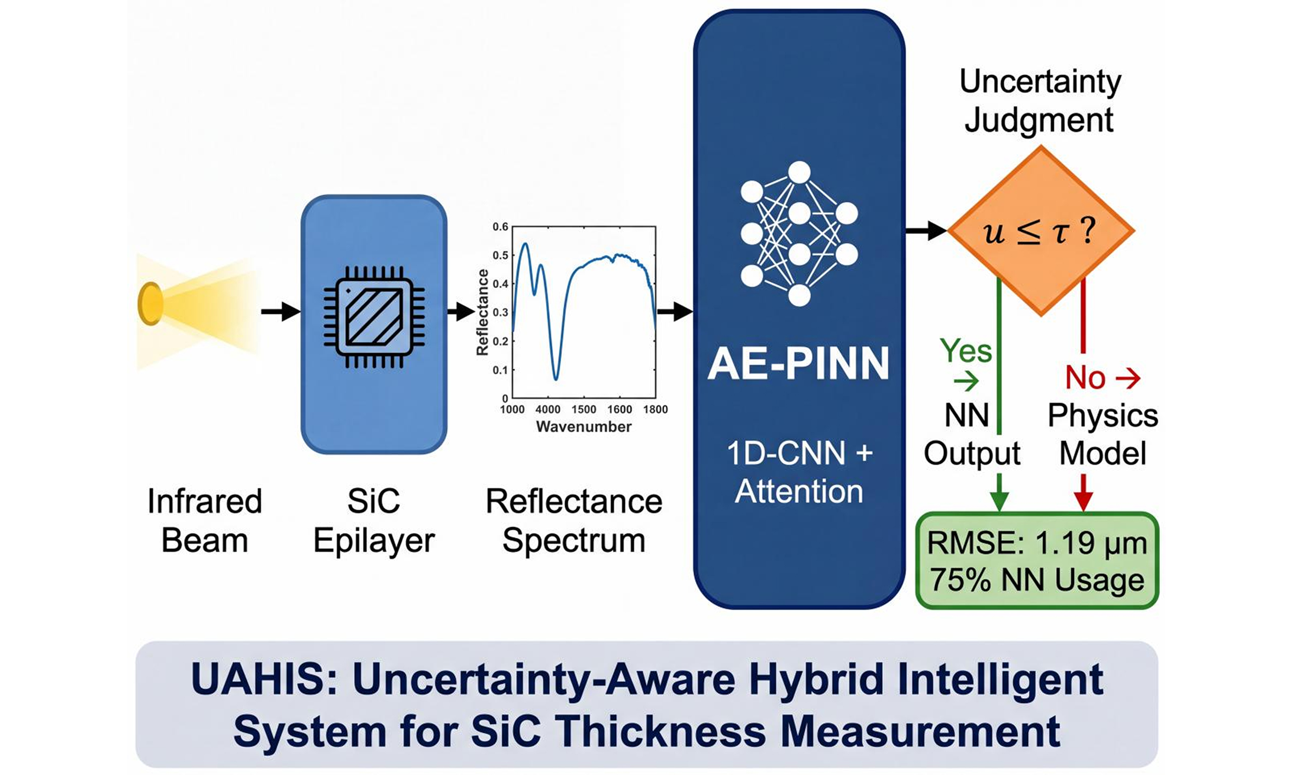
The thickness of silicon carbide (SiC) epilayers critically determines device performance; however, conventional optical methods suffer from low efficiency and limited robustness to noise. We propose an Uncertainty-Aware Hybrid Intelligent System (UAHIS) that integrates a physical benchmark model based on multi-beam interference with an attention-enhanced physics-informed neural network (AE-PINN). Trained on 50,000 real spectra, the AE-PINN serves as a rapid prediction engine, achieving a root mean square error (RMSE) of 1.194 μm for the test set. The Monte Carlo Dropout enables the UAHIS to quantify prediction uncertainty and adaptively switch between neural network prediction and physical model verification. The optimal uncertainty thresholds were 0.391 μm (global), 0.397 μm (SiC), and 0.252 μm (Si). Using real experimental data, the UAHIS achieved a 75.0% AE-PINN utilization rate and a mean absolute error of 0.12 μm for the SiC samples. Under various noise conditions, the average prediction error of the AE-PINN was 23.4% of that of a standalone physical model. An uncertainty-guided incremental learning mechanism further enables the continuous self-optimization of the model. This study offers a unified framework for intelligent optical thin-film thickness measurement, balancing accuracy and adaptability.
Keywords
1. INTRODUCTION
Silicon carbide (SiC), a third-generation wide-bandgap semiconductor, is widely used in power devices for new energy vehicles, rail transportation, and smart grids owing to its high-voltage resistance, high-temperature tolerance, and high-frequency performance[1,2]. Epilayer thickness critically affects device performance metrics, such as the breakdown voltage and on-resistance, making accurate and efficient measurement essential for process monitoring and yield improvements[3]. Consequently, fast and non-contact optical measurement methods are preferred for practical applications in this field.
Infrared interferometry is a well-established technique for measuring optical film thickness. The physical basis of this technique lies in the interference of light reflected at the upper and lower interfaces of the film; the film thickness is retrieved by analyzing the interference fringe period in the reflectance or transmittance spectrum[4]. For example, Mpilitos et al. developed a transmission line model to interpret infrared interference signals to predict the thickness of dielectric films deposited on highly doped substrates, which has been successfully applied to characterize various materials, including SiC[4]. Costantini et al. investigated the temperature dependence of the refractive index of ion-implanted SiC epilayers by analyzing interference fringes in their transmission spectra[2].
However, traditional analytical methods, such as fast Fourier transform or peak-to-peak distance calculation, have inherent limitations: their accuracy relies on the precise extraction of fringe peak and valley positions, making them sensitive to measurement noise[4]. Moreover, they suffer from low computational efficiency when dealing with complex optical models and fail to meet the high-throughput demands of industrial in-line inspections. To address these limitations, we first corrected the unit conversion error in the multibeam interference model and established a high-precision physical benchmark model, providing a reliable theoretical reference and verification standard for the entire measurement system.
In recent years, physics-informed neural networks (PINNs) have provided a new paradigm for solving various scientific computing problems in engineering[5]. PINNs embed the residual of the governing partial differential equation as a soft constraint into the neural network loss function, fusing data-driven learning with physical laws and significantly reducing dependence on large amounts of labeled data. This method has shown great potential in many engineering fields, including solid mechanics, fluid mechanics, heat transfer, and mass transfer. For instance, in solid mechanics, Li et al. used PINNs to analyze laminated glass behavior[6]; Wang et al. proposed a mesh-based PINN for linear elasticity[7]; Ouyang et al. extended PINNs to pile deflection analysis[8]; and Ye et al. combined PINNs with Fourier networks for damping modeling[9]. In fluid mechanics, Peng et al. developed a physics-informed graph convolutional network for flow fields[10]; Zhao et al. proposed an adaptive PINN solver for heat flow[11]; Cheng et al. integrated ResNet into PINNs for Navier-Stokes solutions[12]; Rui et al. applied PINNs for 3D flow reconstruction[13]; Jalili et al. used PINNs for two-phase heat transfer[14]; and Yadav et al. proposed reactive-flow physics-informed neural networks (RF-PINNs) for flame-field reconstruction[15]. In mass transfer and other cross-disciplinary areas, Batuwatta-Gamage et al. applied PINNs for the first time to model mass transfer during plant cell drying, achieving errors below 0.33%[16]. Furthermore, researchers have attempted to apply PINNs to more complex scenarios, such as computing blood flow through transcatheter aortic valve implantation devices[17] and solving electrothermal multi-physics coupling problems[18]. Wang et al. proposed a physics-data-driven method to predict surface and building settlements induced by tunnel construction[19]. Chen et al. applied PINNs to estimate highway traffic states using sparse observation data[20]. To further enhance the performance and applicability of PINNs, researchers have developed various improved architectures, such as the physics-informed convolutional recurrent network (PhyCRNet)[21], discussions on combining PINNs with traditional linear solvers[22], modified PINNs for predicting vector optical solitons in birefringent fibers[23], flow data assimilation[24], extended physics-informed neural networks (XPINNs) for space-time domain decomposition[25], and the discovery of variable-order fractional models for turbulent Couette flow[26]. Recently, Qian et al. conducted an in-depth study on error analysis and algorithm improvements for PINNs, providing theoretical guarantees for their application in solving dynamic partial differential equations (PDEs)[27,28]. Liu et al. extended PINNs to solve the neutron transport equation and demonstrated their potential in complex physical systems[29]. Additionally, Son et al. used PINNs to identify noise-driven dynamic parameters in thermoacoustic systems, demonstrating their capabilities in a stochastic environment[30].
Despite the widespread success of PINNs in many scientific computing fields, their direct application to high-precision and high-robustness SiC epilayer thickness measurements still faces three challenges. First, most existing PINN studies are validated in simulations or controlled environments, lacking targeted optimization for spectral feature extraction in the complex noisy environments of industrial measurements, resulting in insufficient noise robustness in real-world scenarios. Second, standard PINNs typically provide only point estimates and lack the ability to quantify prediction uncertainty; thus, they fail to provide confidence assessments for the measurement results, posing a decision risk in practical applications. Third, a single PINN model may suffer from accuracy degradation when processing high-frequency interference fringes, and training/inference can be time-consuming, making it difficult to simultaneously meet the robustness and accuracy requirements of industrial in-line inspections. Achieving an intelligent balance between the two is a key challenge in this field. An ideal measurement system must achieve an intelligent trade-off between robustness, accuracy, and reliability.
To address these challenges, we propose an Uncertainty-Aware Hybrid Intelligent System (UAHIS), whose core is an attention-enhanced physics-informed neural network (AE-PINN). The system uses AE-PINN for fast prediction and quantifies the prediction uncertainty; when the uncertainty exceeds a threshold, it automatically switches to a high-precision physical model for verification, thereby maximizing efficiency while ensuring accuracy. Furthermore, the system incorporates an incremental learning mechanism based on uncertainty Awareness, enabling continuous self-improvement using samples collected during actual measurements, which triggers physical model verification. The main contributions of this study are as follows:
1. We designed the AE-PINN by introducing a channel attention mechanism to focus on key spectral features and a spectral consistency physical constraint loss, which significantly improved the prediction accuracy and noise robustness for thick-layer samples.
2. We propose a hybrid decision framework based on Monte Carlo dropout uncertainty quantification, which integrates an uncertainty-Aware, incremental learning mechanism. The system can automatically evaluate the confidence of AE-PINN predictions and intelligently switch between the “AE-PINN fast prediction” and “physical model accurate verification” modes using material-adaptive thresholds, while continuously self-optimizing using samples collected during actual measurements that trigger the physical model verification, fundamentally ensuring the unity of efficiency, accuracy, and long-term adaptability.
The remainder of this paper is organized as follows: Section 2 describes the high-precision physical benchmark model; Section 3 details the construction of AE-PINN and its integration with the physical model in UAHIS; Section 4 presents the experimental results and analysis; and Section 5 concludes the paper and discusses future work.
2. HIGH-PRECISION PHYSICAL BENCHMARK MODEL
2.1. Measurement principle
The basic principle of measuring the SiC epilayer thickness using infrared interferometry is illustrated in Figure 1. A broad-spectrum infrared beam was incident on the sample surface at an angle of α. Reflections occur at the air-epilayer and epilayer-substrate interfaces, and the two reflected beams interfere, forming interference fringes that vary with wavelength.
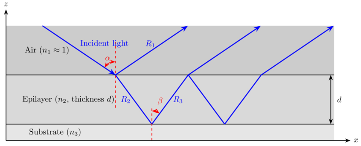
Figure 1. Schematic diagram of the multi-beam interference measurement principle (incident angle α and refraction angle β are marked).
2.2. Multi-beam interference theoretical model
According to Snell’s law, the incident angle α and refraction angle β satisfy:
where n0 is the refractive index of air (approximately 1); n is the refractive index of the epilayer; and α is the incident angle; β is the refraction angle.
The optical path difference between adjacent reflected beams is:
where ΔL is the optical path difference; d is the epilayer thickness.
The corresponding phase difference is:
where δ is the phase difference; λ is the wavelength of the incident light.
Using the amplitude superposition method to derive the reflectance formula for multi-beam interference, we define the amplitude reflection coefficients r12, r23 and amplitude transmission coefficients t12, t23, satisfying the Stokes relations:
where r12 and t12 are the amplitude reflection and transmission coefficients at the air-epilayer interface; r23 and t23 are the amplitude reflection and transmission coefficients at the epilayer-substrate interface.
Under the simplifying assumption r12 ≈ r23 = r, the total reflected amplitude is the coherent superposition of all reflected beams, yielding the Airy formula[4]:
where R(δ) is the reflectance; F is the coefficient of finesse.
The coefficient of finesse F is defined as:
where R is the reflectance; r is the amplitude reflection coefficient.
During the implementation of the physical model, we unified the wavelength λ in the original model. The correct phase difference formula after unit correction is:
where
In the original formulation, the wavelength λ was used directly in the phase difference formula without proper unit conversion, leading to dimensional inconsistencies when calculating thicknesses greater than
According to the Airy formula, the reflectance reaches a maximum when sin2(δ/2) = 1, corresponding to the phase condition δ = (2m + 1)π. Substituting into Equation (3) yields:
where m is the interference order (m = 0, 1, 2, …).
For two adjacent interference peaks, the corresponding wavenumbers are
where
Subtracting these two equations yields the wavenumber difference between the adjacent interference peaks:
where Δ
Therefore, we obtain the thickness formula independent of the interference order:
where d is the epilayer thickness; Δ
Here cosβ can be calculated from Equation (1):
where cosβ is the cosine of the refraction angle; α is the incident angle; n is the epilayer refractive index.
This physical model provides a theoretical foundation for the subsequent neural network training and also offers a reliable high-precision verification method for the UAHIS.
3. AE-PINN AND HYBRID INTELLIGENT MEASUREMENT SYSTEM
Although traditional physical models are accurate, they suffer from low computational efficiency and cannot meet real-time measurement requirements. To overcome this bottleneck, we constructed an AE-PINN surrogate model to achieve an end-to-end fast prediction of epilayer thickness from interference spectra. This model integrates large-scale real data acquisition and labeling, a spectral attention mechanism, an indirect physical constraint loss function, and Monte Carlo Dropout uncertainty quantification modules, achieving efficient prediction while maintaining physical consistency and enabling evaluation of prediction reliability.
To illustrate the complete flow of the proposed AE-PINN algorithm more clearly, Figure 2 shows the overall flowchart. The algorithm comprises four core phases: (1) real data acquisition and preprocessing; (2) AE-PINN model training; (3) physical constraint mechanism; and (4) uncertainty-Aware hybrid decision-making.
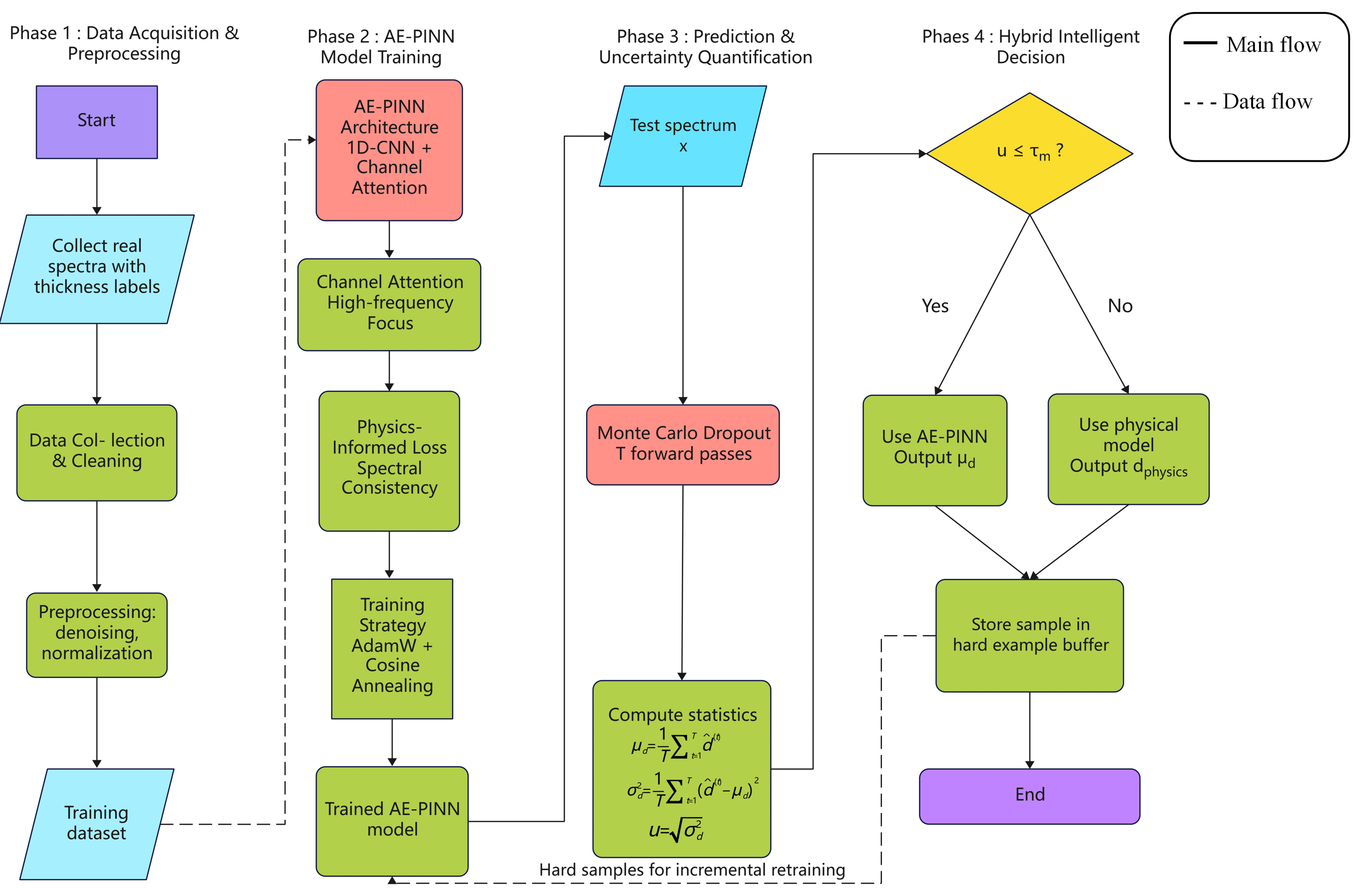
Figure 2. Flowchart of the AE-PINN algorithm. The algorithm consists of four core phases: (1) Real data acquisition and preprocessing: collect real interference spectra with thickness labels, and build the training set through denoising and normalization; (2) AE-PINN model training: includes 1D-CNN, channel attention module, and training with physical constraints; (3) Physical constraint mechanism: implement physical constraints through spectral consistency checking; (4) Uncertainty-Aware hybrid decision: intelligent mode switching based on uncertainty quantification via Monte Carlo Dropout. AE-PINN: Attention-enhanced physics-informed neural network; 1D-CNN: one-dimensional convolutional neural network.
These four phases are interconnected, forming a complete closed-loop system: starting from real data acquisition, making predictions through the AE-PINN architecture, ensuring physical consistency using the physical constraint mechanism, and finally deciding whether to use the neural network prediction or switch to the physical model based on the uncertainty assessment.
3.1. AE-PINN surrogate model
3.1.1. Network architecture design
The AE-PINN employs a deep convolutional encoder design optimized for the spectral characteristics of the interference spectra. Let the input spectral data be x ∈ RN, where N is the number of wavelength points (specific value given in Section 4.1). The entire encoder is stacked in four convolutional stages, with kernel sizes denoted as K1, K2, K3, K4 and output channels denoted as C1, C2, C3, C4 (specific values listed in Section 4.1). Each stage sequentially performs a one-dimensional convolution, batch normalization, and nonlinear activation, with max pooling inserted before the second to fourth stages to downsample the feature maps.
First, for the l-th convolution layer, the input feature map is denoted as F(l-1) ∈
where the output feature length Ll is determined by the input length Ll-1, kernel size Kl, padding pl, and stride sl:
In this study, all convolutional layers used zero padding (pl = 0), the main convolution stride was sl = 1, and the equivalent stride for pooling was sl = 2, implemented via strided convolutions instead of explicit pooling layers.
Subsequently, batch normalization is applied to the convolution output Z(l). For a mini-batch containing m samples B = {z1, z2, …, zm}, batch normalization performs the following transformation independently for each channel:
where ϵ = 10-5 is a small constant to avoid division by zero; γ,β ∈
The activation function is the rectified linear unit, defined mathematically as
This function offers sparse activation and alleviates the vanishing gradient problem; ϕR(·) denotes the rectified linear unit (ReLU) activation.
Before the second to fourth layers, we introduced max pooling to reduce the size of the feature maps. For a max pooling operation with a window size of 2 and stride 2, the operation is defined as
where ϕP denotes the max pooling function, which halves the feature length while preserving locally salient features.
Based on the basic operators above, the complete forward pass of the four-layer convolutional encoder can be expressed as follows. First layer:
Second layer (with pooling):
Third layer (with pooling):
Fourth layer (with pooling):
where * denotes the discrete convolution defined in Equation (14), ϕP is applied according to Equation (18), ϕBN according to Equation (16), and ϕR according to Equation (17).
After this encoding, the original spectrum x ∈ RN is mapped to a high-dimensional feature map F(4) ∈
In terms of the training strategy, the AE-PINN uses the AdamW optimizer, along with cosine annealing learning rate scheduling and gradient clipping to prevent training instability. Weight initialization employs Kaiming normal initialization to accelerate convergence. The specific training hyperparameters (e.g., initial learning rate, batch size, and number of epochs) are provided in Section 4.1.
3.1.2. Spectral attention mechanism
Different wavelength regions in an interference spectrum have varying importance in thickness estimation. Based on physical principles, larger thicknesses correspond to higher fringe frequencies. To guide the network to adaptively focus on high-frequency features, we introduced a channel attention module after the convolutional encoder.
Let F(4) ∈ RC×H be the feature map output from the fourth layer, where C = C4 is the number of channels and H = L4 is the spatial dimension. First, GAP and global max pooling (GMP) are used to aggregate global information per channel:
The two pooled results are concatenated and fed into a gating mechanism consisting of two fully connected layers to generate a channel weight vector A ∈ RC. The dimensions of the two fully connected layers are controlled by a reduction ratio r, i.e., W1 ∈
where [·;·] denotes concatenation, σ is the sigmoid activation function, and ϕR is the ReLU activation defined in Equation (17). Finally, the channel weights A are multiplied element-wise back to the original feature map to achieve feature recalibration:
where
This operation enables the network to adaptively enhance high-frequency channels and suppress low-frequency channels, thereby improving the prediction accuracy for thick-layer samples. The design philosophy of this attention mechanism aligns with recent research on the use of attention for feature fusion in point cloud segmentation[31]and model-based deep learning for image fusion[32].
To provide an intuitive insight into the attention mechanism, we visualized the channel attention weights [Figure 3]. The figure shows the distribution of attention weights across the 512 channels, with higher weights indicating more informative spectral features. Specifically, the attention weights were sorted in descending order, and the cumulative sum of the sorted weights was computed. The number of channels required to reach 90% of the total cumulative weight was identified. The cumulative distribution reveals that the top 90% of the attention mass is concentrated in approximately 200 channels, demonstrating that the attention mechanism effectively focuses on a subset of frequency bands relevant to thickness prediction while suppressing less informative channels.
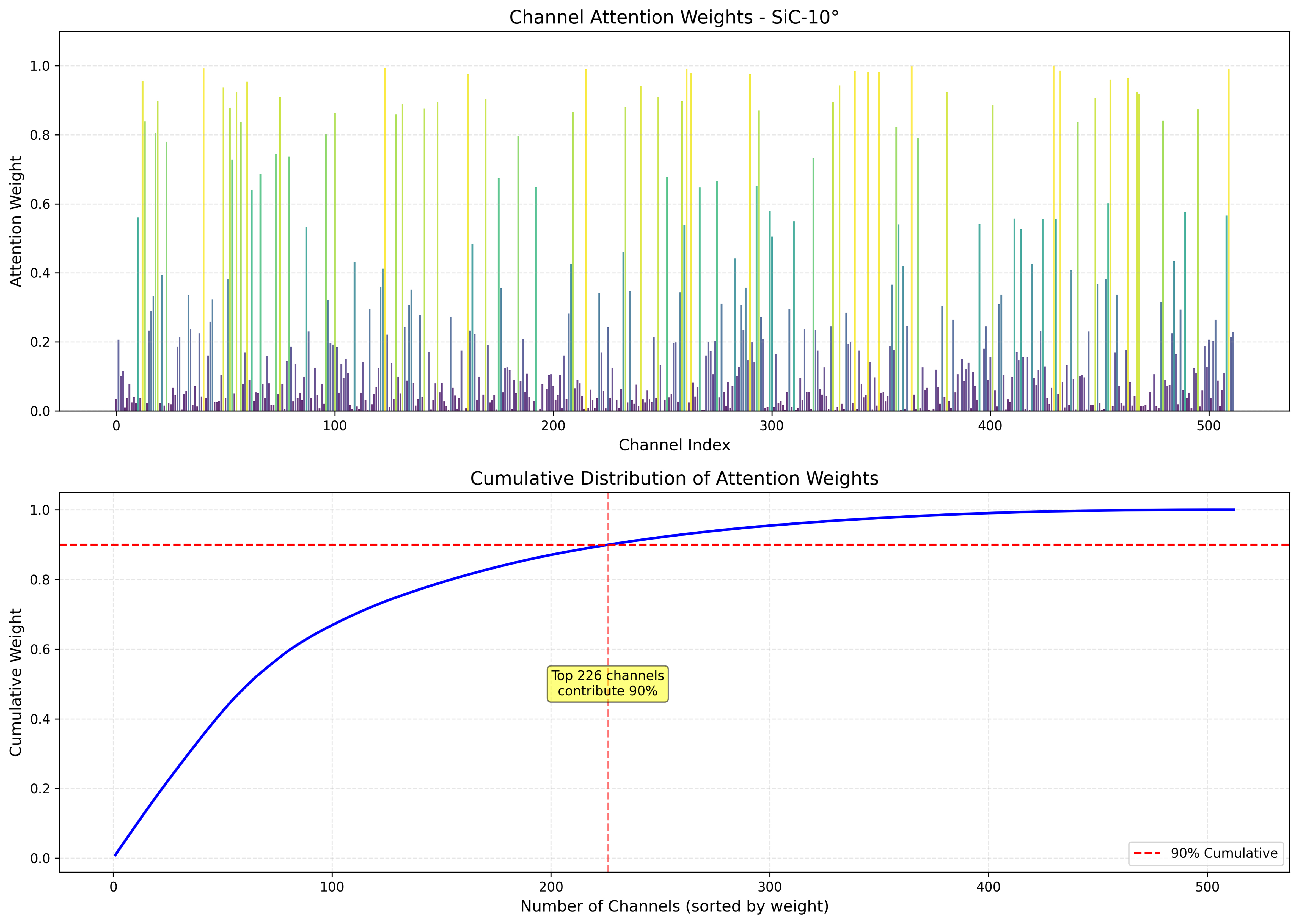
Figure 3. Channel attention weight distribution of the AE-PINN. The top panel shows the attention weight for each of the 512 channels, and the bottom panel shows the cumulative distribution. Approximately 200 channels contribute 90% of the total attention mass. AE-PINN: Attention-enhanced physics-informed neural network; SiC: silicon carbide.
3.1.3. Indirect physical constraint loss function
We propose an innovative spectral consistency physical constraint. According to multi-beam interference theory, the thickness d is proportional to the interference fringe frequency f:
For samples with larger thicknesses (we set a thickness threshold dth, whose specific value is given in Section 4.1), the interference fringes are denser, and the energy of high-frequency components in the Fourier spectrum should be higher. Based on this physical principle, we designed a physical constraint loss term:
where Etotal,i is the total spectral energy, Ehigh,i is the high-frequency energy, I() is the indicator function, and ϕR is the ReLU function defined in Equation (17). The complete loss function is:
where LMSE is the standard mean squared error loss, and the balancing coefficient λ is determined experimentally.
3.1.4. Monte Carlo Dropout uncertainty quantification
To provide reliable decision-making for UAHIS, the AE-PINN employs the Monte Carlo Dropout method for uncertainty quantification. The core idea is to keep the dropout activated during inference and estimate the prediction uncertainty through multiple stochastic forward passes. The specific implementation is as follows: For the trained AE-PINN model, the dropout layers were kept active during inference. For the same input spectrum x, T stochastic forward passes are performed, each time randomly dropping out a subset of neurons, yielding a set of slightly different predictions {
Based on these T predictions, the statistical properties of the thickness prediction are calculated:
where μd is the mean prediction, i.e., the final thickness estimate; σd2 is the prediction variance, reflecting the dispersion of the predictions; u is the standard deviation, i.e., the uncertainty measure. A smaller u indicates higher confidence in the prediction for that sample, with the multiple predictions being more concentrated; conversely, a larger u indicates greater uncertainty, with predictions more spread out, possibly due to the sample lying outside the training distribution or being affected by noise.
Based on the uncertainty u, the system sets an uncertainty threshold τ for intelligent decision-making. The decision rule can be expressed as:
The choice of threshold τ is based on a statistical analysis of the prediction uncertainty distribution for different materials. By analyzing the neural network uncertainty distribution in the validation set, we found that the optimal threshold differed between materials. For SiC and Si, we set material-specific adaptive thresholds, enabling the system to adjust intelligently according to the optical properties of different materials and avoid performance loss that could result from a fixed threshold.
When the uncertainty u of the AE-PINN prediction is less than or equal to the threshold τ, the system considers the prediction sufficiently reliable and directly adopts the AE-PINN result, leveraging its millisecond-level fast prediction capability. When s exceeds τ, the system recognizes that the neural network prediction is highly uncertain and automatically switches to the high-precision physical model for verification, ensuring measurement accuracy.
Through this uncertainty-Aware architecture, the AE-PINN not only provides thickness predictions but also evaluates its own reliability, offering critical information for subsequent intelligent decisions by the UAHIS. This design enables the system to identify and handle samples outside the training distribution, significantly enhancing robustness and reliability, providing an important safeguard for practical industrial applications.
3.2. UAHIS: Uncertainty-Aware Hybrid Intelligent System
Traditional numerical methods suffer from low computational efficiency and strong dependence on boundary conditions when dealing with complex physical models. Although fast, purely data-driven neural networks can produce unreliable predictions outside the training distribution and lack interpretability. To overcome these limitations, we propose an UAHIS that combines the efficient prediction capability of AE-PINN with the accurate computational advantage of a physical model. By quantifying the prediction uncertainty, the system intelligently switches between the two modes, significantly improving the computational efficiency while ensuring measurement accuracy. Similarly, in advanced control fields, quantifying and compensating for system uncertainty using disturbance observers has been proven effective for enhancing robustness[33]. This study draws on this idea and uses quantified prediction uncertainty to guide intelligent decisions in the system.
3.2.1. System working principle and architecture
The core design idea of the UAHIS is to use AE-PINN for fast initial prediction while simultaneously quantifying the prediction uncertainty via the Monte Carlo Dropout method (detailed in Section 3.1.4), and then decide whether to invoke the physical model for verification based on an uncertainty threshold. Figure 4 shows the complete flowchart of the system.
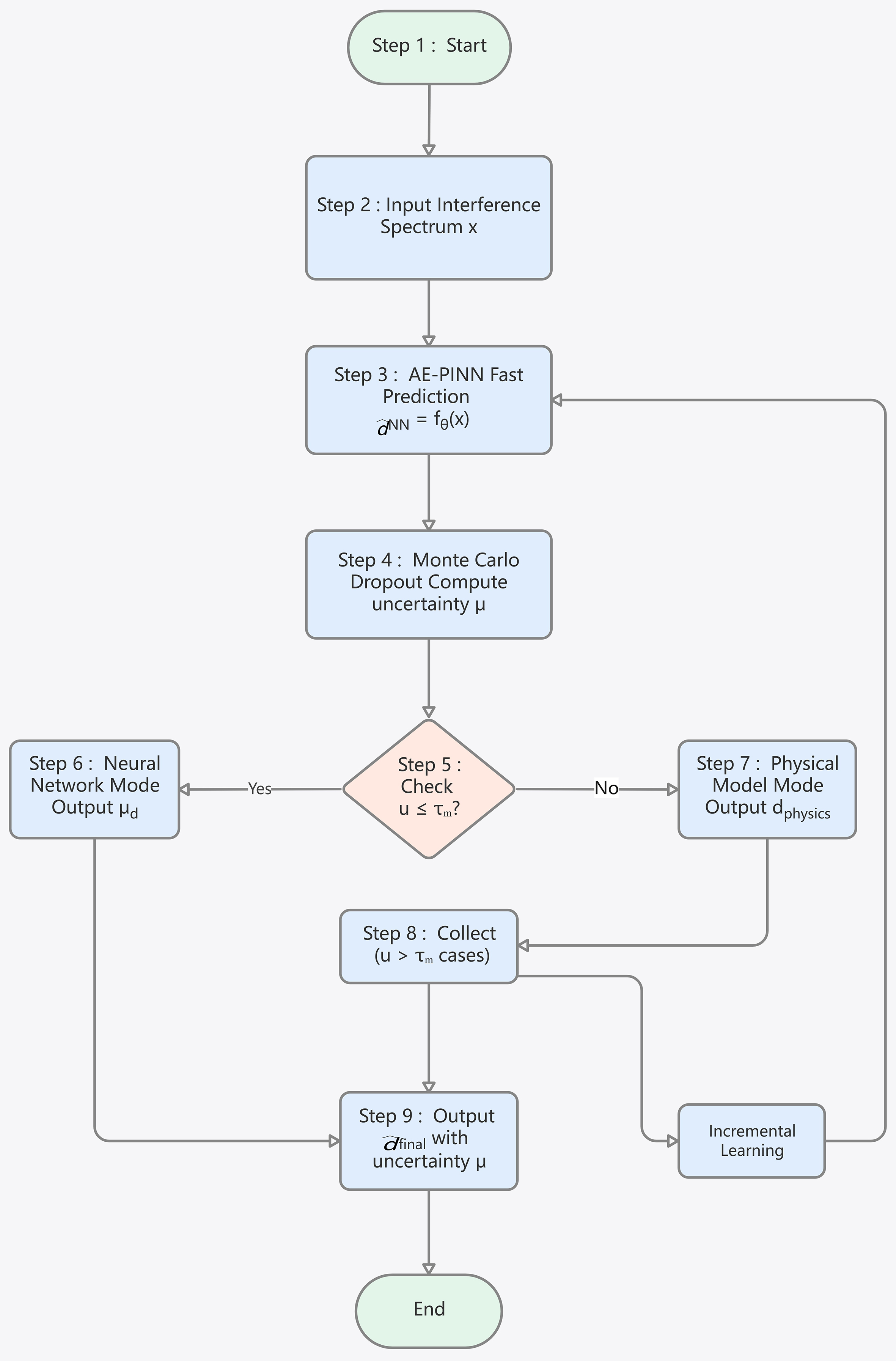
Figure 4. Algorithm flowchart of the UAHIS. τm is the material-specific threshold, and u is the prediction uncertainty obtained from Monte Carlo Dropout. UAHIS: Uncertainty-Aware Hybrid Intelligent System; AE-PINN: attention-enhanced physics-informed neural network.
The system first receives the interference spectrum of the sample to be measured and makes a rapid thickness prediction using the pre-trained AE-PINN. Unlike traditional neural networks, we used the Monte Carlo Dropout method during inference, performing multiple forward passes and quantifying the prediction uncertainty by analyzing the distribution of the results. This uncertainty measure reflects the model’s confidence in its prediction for the current sample, providing a quantitative basis for subsequent mode selection.
3.2.2. Adaptive threshold decision mechanism
The core decision rule of the hybrid system is based on the uncertainty threshold τ: when the AE-PINN prediction uncertainty u ≤ τ, the system adopts the fast AE-PINN prediction result; otherwise, it switches to the high-precision physical model for verification. The formal expression of this decision rule and the threshold optimization method are detailed in Section 3.1.4 (under “Uncertainty threshold decision”) and will not be repeated here.
We further introduced a material-specific adaptive threshold strategy. Given the differences in the optical properties of the materials, the system sets independent optimal thresholds for each material based on the statistical characteristics of the uncertainty distribution on the validation set. This strategy enables the system to dynamically adjust the decision boundary according to the optical properties of the measured object, effectively avoiding the performance loss associated with a single fixed threshold when applied across materials and significantly enhancing the environmental adaptability and robustness of the UAHIS. The specific threshold values are provided in Section 4.3.
The computational cost of the hybrid system is dominated by the AE-PINN inference with the Monte Carlo Dropout, which requires 30 forward passes per sample. On a standard CPU (Intel Core i7-12700H), the average inference time for the AE-PINN was 164.74 ms per sample, whereas the physical model required 21.57 ms per sample. Although the physical model is faster for single inference, it exhibits poor robustness and is strongly affected by peak selection and noise. Within this hybrid system, 75.0% of samples can be processed by AE-PINN, substantially reducing reliance on the physical model.
3.2.3. Incremental learning and system self-optimization
To cope with new sample distributions, changing noise patterns, or material property drifts that may occur in practical applications, we designed an incremental learning framework based on uncertainty Awareness. The core idea of this mechanism is to use the “challenging samples” that trigger the physical model verification in UAHIS to periodically fine-tune the AE-PINN, gradually adapting it to new data distributions and improving its predictive capability on edge cases.
When the system detects that a sample’s prediction uncertainty exceeds the threshold τ, it automatically switches to the physical model for verification and marks this sample along with its physical model prediction dphys as a “challenging sample”, which is stored in a buffer. Periodically, the collected samples are used to fine-tune the AE-PINN, forming an incremental learning dataset Dinc = {(xi, diphys)}i=1N.
Incremental learning fine-tunes the pre-trained AE-PINN model using the following loss function:
During fine-tuning, the learning rate was set to a low value, and the number of epochs was kept small to avoid catastrophic forgetting. The specific fine-tuning hyperparameters are explained in Section 4.6. After fine-tuning, the updated model was redeployed into the system, replacing the original AE-PINN module, thereby achieving continuous system optimization.
4. EXPERIMENTAL RESULTS AND ANALYSIS
4.1. Experimental setup
Dataset: We collected 50,000 real measured spectra to train and validate the AE-PINN model, covering both SiC and Si materials. All spectra were obtained using a Fourier-transform infrared (FTIR) spectrometer (Nicolet iS50, Thermo Fisher Scientific) equipped with a reflectance accessory. The measurements were performed at room temperature with a spectral resolution of 4 cm-1 over the wavenumber range of 400-
A typical reflectance spectrum of a SiC sample is shown in Figure 5. The spectrum exhibits clear interference fringes with regularly spaced peaks, which are the basis for thickness determination. The peak positions are annotated in the figure, illustrating the characteristic interference pattern used by both the physical model and the neural network.
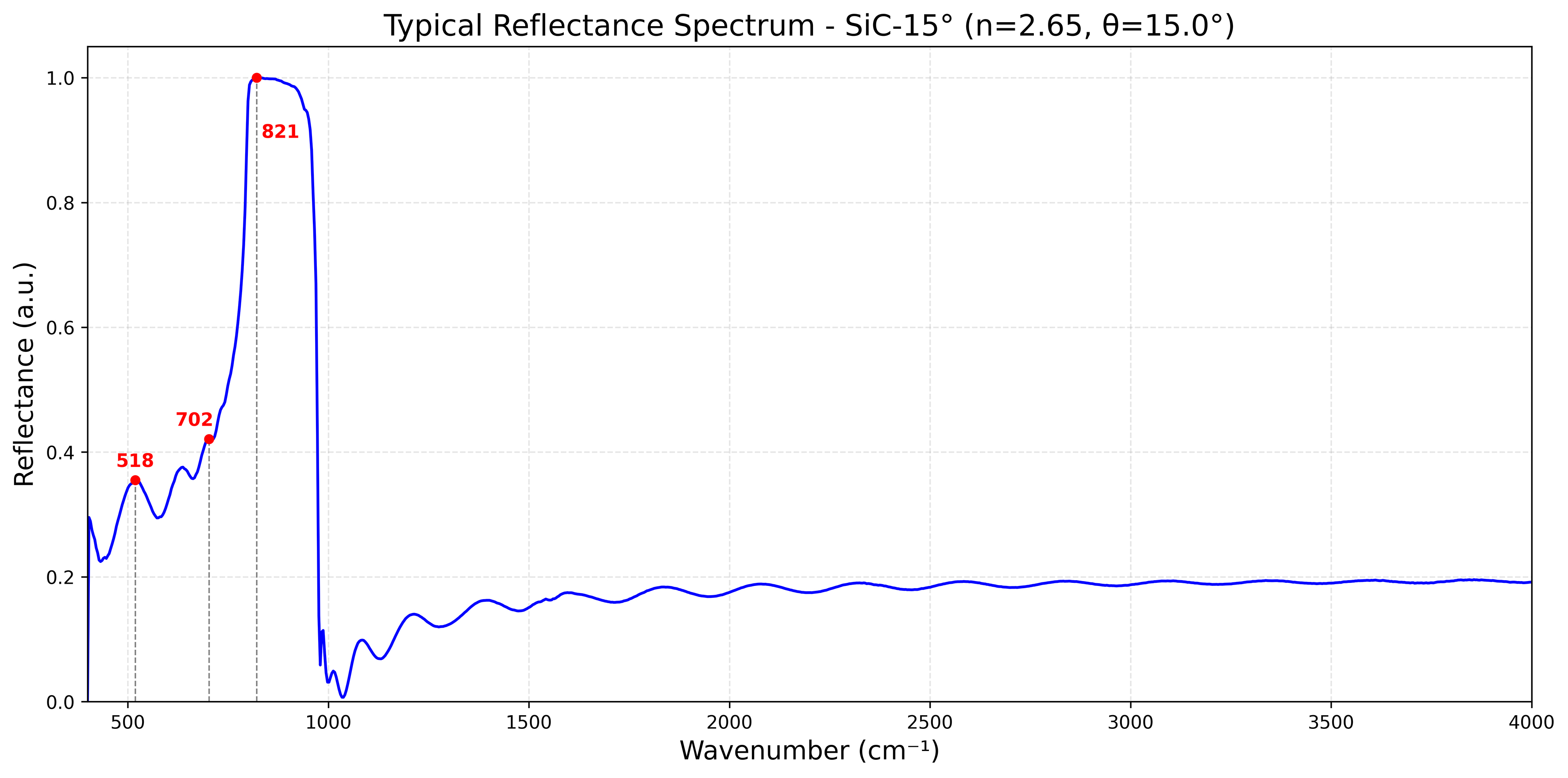
Figure 5. Typical reflectance spectrum of a SiC epilayer sample measured over the wavenumber range of 400-4,000 cm-1. Interference peaks are annotated with their corresponding wavenumber positions. SiC: Silicon carbide.
All spectra were normalized as follows:
where μx and σx are the mean and standard deviation of the sample spectrum, respectively. Additionally, 4 independent real samples were collected to test the performance of the UAHIS in real-world scenarios.
The input to the neural network was the normalized reflectance spectrum, represented as a 1000-dimensional vector corresponding to the wavenumber range of 400-4,000 cm-1. The ground-truth thickness labels for training were obtained by applying the physical model (Section 2.2) to each measured spectrum, with the model parameters (refractive index n and incidence angle α) determined from the sample specifications. The dataset was randomly partitioned into training, validation, and test sets in a 70:15:15 ratio, ensuring that the test set was not used in any stage of model selection or hyperparameter tuning.
Network Architecture Parameters: The number of input spectral points for the AE-PINN was set to N = 1,000. The kernel sizes of the four convolutional layers were K1 = 15, K2 = 11, K3 = 7, K4 = 5; the output channels were C1 = 64, C2 = 128, C3 = 256, C4 = 512. The reduction ratio for the attention mechanism was r = 16. The thickness threshold in the physical constraint loss was dth = 10 μm, which corresponds to the minimum thickness of the thick-layer samples, ensuring the effectiveness of the constraint.
Training Hyperparameters: AE-PINN is trained using the AdamW optimizer with an initial learning rate of 10-3 and a weight decay of 10-4. The learning rate schedule employs a cosine annealing restart strategy with a minimum learning rate of 10-6. Gradient clipping was applied with a maximum norm of 1.0. The batch size was 64, and the model was trained for 200 epochs. All hyperparameters were determined using a via grid search on the validation set.
Uncertainty Quantification Parameters: The number of forward passes for Monte Carlo Dropout is T = 30, determined experimentally as the point where the variance of the uncertainty estimate stabilizes, providing a trade-off between computational cost and stability.
Incremental Learning Parameters: For incremental fine-tuning, the learning rate was set to 10-4 and the number of epochs to 10 to avoid catastrophic forgetting.
Hardware and software environment: Intel Core i7-12700H processor, NVIDIA GeForce RTX 3060 GPU
4.2. AE-PINN training results
The initial training result of the baseline AE-PINN without ablation was root mean square error (RMSE) = 1.4802 μm. After unified training under the ablation experiment settings, the complete AE-PINN model achieved RMSE = 1.1943 μm on the test set, with mean absolute error (MAE) = 1.0045 μm and coefficient of determination (R2) = 0.9523, indicating that the model accurately explains 95.2% of the thickness variation. Notably, the prediction accuracy for thick-layer samples with thicknesses greater than dth is significantly improved, thanks to the introduction of the physical constraint loss, which enables the model to learn the intrinsic physical relationship between fringe frequency and thickness during training. The attention mechanism allows the model to effectively identify key interference features in the spectrum, suppress noise interference, and enhance robustness and generalization. The balancing coefficient λ = 0.1 for the physical constraint loss was determined via grid search on the validation set, sampling logarithmically from 0.01 to 1.0 and selecting the value that minimized the RMSE on the validation set.
To comprehensively evaluate the performance of the AE-PINN, we summarize its core performance metrics on the test set in Table 1. The results demonstrate that the model excels in all three core dimensions of thickness prediction, validating the effectiveness of the proposed enhanced architecture.
Core performance metrics of AE-PINN
| Metric | Value | Unit |
| RMSE | 1.1943 | μm |
| MAE | 1.0045 | μm |
| R2 | 0.9523 | - |
To further validate the effectiveness of each component, we conducted ablation experiments by training five variants under identical conditions: (1) Full AE-PINN (complete model with attention and physical constraints); (2) No Attention (remove channel attention module); (3) No Hybrid Strategy (remove the hybrid switching mechanism, using only neural network predictions); (4) No Physics Loss [remove the physical constraint loss, retaining only mean squared error (MSE) loss]; and (5) Baseline convolutional neural network (CNN, remove both attention and physical constraints). The results are presented in Table 2. The full AE-PINN achieved the lowest RMSE (1.1943 μm), outperforming all variants. Removing the attention mechanism led to a 4.1% degradation, removing the hybrid strategy led to a 5.0% degradation, and removing the physical constraint loss led to an 18.5% degradation. The Baseline CNN, which lacks both attention and physical constraints, shows the largest degradation of 21.4%. These results confirm that each component contributes positively to the overall performance, with the physical constraint providing the most significant improvements.
Ablation study results of AE-PINN variants
| Model | RMSE (μm) | MAE (μm) | R2 | Relative degradation |
| Full AE-PINN | 1.1943 | 1.0045 | 0.9523 | - |
| No Attention | 1.2452 | 1.0491 | 0.9482 | 4.10% |
| No Hybrid Strategy | 1.2535 | 1.0562 | 0.9473 | 5.00% |
| No Physics Loss | 1.4148 | 1.1996 | 0.9334 | 18.50% |
| Baseline CNN | 1.5198 | 1.2258 | 0.9236 | 21.40% |
The training and validation loss curves, as well as the correlation between predicted and true thicknesses, are shown in Figure 6. The figure shows that the model converged stably after approximately 120 epochs, with no significant overfitting. It is worth noting that the prediction errors are slightly larger in the low-frequency region of the spectrum (wavenumber < 1,000 cm-1), which we attribute to the reduced fringe density in this range. The physical constraint loss [Equation (27)] partially compensates for this by enforcing the relationship between fringe frequency and thickness; however, the overall accuracy in this region remains slightly lower than that in the mid- and high-frequency regions.
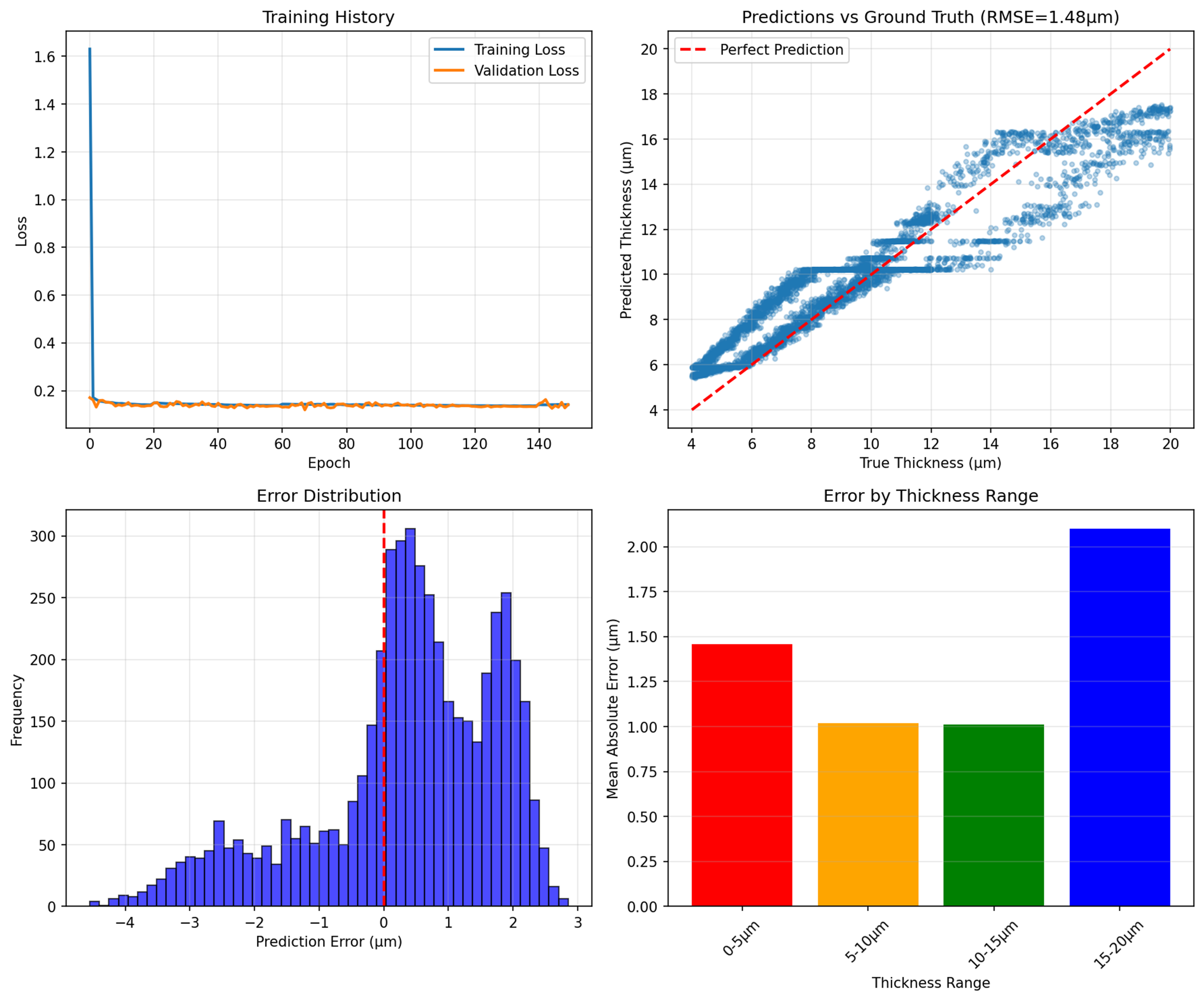
Figure 6. Visualization of AE-PINN training results. AE-PINN: Attention-enhanced physics-informed neural network.
4.3. Threshold optimization and sensitivity analysis
To determine the optimal uncertainty threshold, we performed a statistical analysis of the prediction uncertainty of the AE-PINN in the validation set. The number of Monte Carlo Dropout forward passes T = 30 has already been explained in Section 4.1 and will not be repeated here.
First, we computed the prediction uncertainty u for all samples in the validation set, and its distribution characteristics are listed in Table 3. The minimum prediction uncertainty was 0.2044 μm, the maximum was 0.4288 μm, the mean was 0.3088 μm, and the median was 0.3011 μm, exhibiting a typical skewed distribution. The 25th percentile was 0.2758 μm, the 75th percentile was 0.3341 μm, and the 90th percentile was
Distribution characteristics of AE-PINN prediction uncertainty
| Statistic | Value (μm) | Description |
| Minimum | 0.2044 | Uncertainty of most certain predictions |
| 25th percentile | 0.2758 | Low-uncertainty samples |
| Median | 0.3011 | Moderate uncertainty |
| 75th percentile | 0.3341 | High-uncertainty samples |
| 90th percentile | 0.3909 | Very high-uncertainty samples |
| Maximum | 0.4288 | Uncertainty of most uncertain prediction |
| Mean | 0.3088 | Average uncertainty level |
Correlation analysis between error and uncertainty shows that the Pearson correlation coefficient between the prediction error |dpred - dtrue| and uncertainty u is 0.6538, while the Spearman rank correlation coefficient reaches 0.9815. This strong correlation indicates that our proposed Monte Carlo Dropout method accurately reflects the reliability of AE-PINN predictions, providing a scientific basis for subsequent threshold decisions.
Threshold sensitivity analysis systematically evaluates the impact of different thresholds τ on system performance, using metrics including AE-PINN usage rate NN_rate(τ), average prediction error Error(τ), and physical model invocation rate Phys_rate(τ). By constructing the objective function NN_rate(τ)-λ·Error(τ) and maximizing it, we achieved an optimal balance between efficiency and accuracy, where the trade-off parameter λ = 10 was determined via a grid search.
As shown in Figure 7, we tested four candidate thresholds: 0.276, 0.301, 0.334, and 0.391 μm. When the threshold is set to 0.391 μm, the AE-PINN usage rate reaches 75%, the physical model invocation rate is 25.0%, and the average prediction error is 0.2153 μm, achieving the best trade-off between efficiency and accuracy. Therefore, we selected τ* = 0.391 μm as the optimal global threshold.
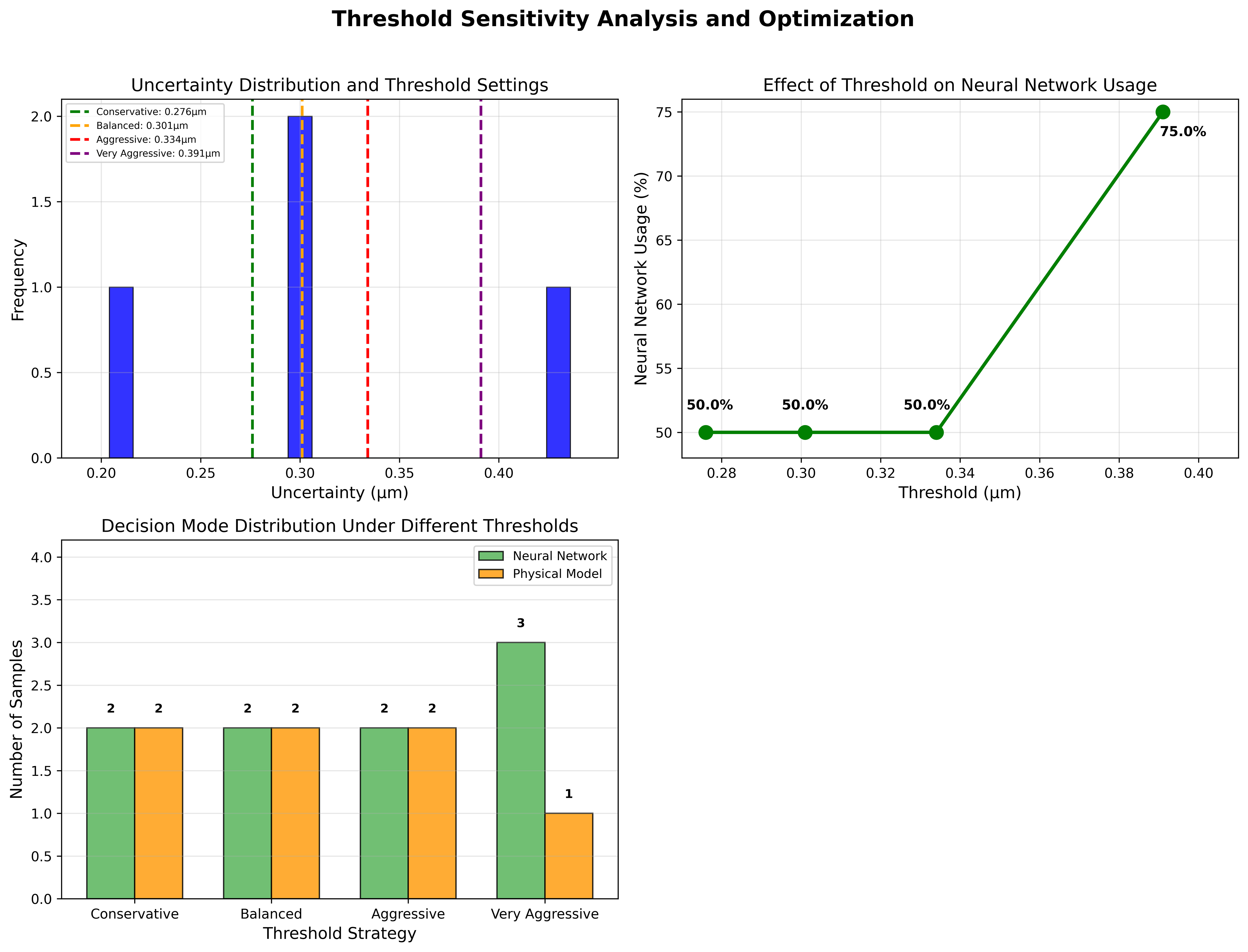
Figure 7. Threshold sensitivity analysis: AE-PINN usage rate and prediction error vs. threshold. AE-PINN: Attention-enhanced physics-informed neural network.
The optimal threshold (0.391 μm) is selected at approximately the 90th percentile of the uncertainty distribution (0.3909 μm), which represents a statistically principled balance between efficiency (maximizing AE-PINN usage) and accuracy (ensuring reliability).
For material-specific adaptive thresholds, we independently optimized the thresholds for SiC and silicon (Si) using their respective validation sets, obtaining τSiC = 0.397 μm and τSi = 0.252 μm. These thresholds are near the 75th percentile of the uncertainty distributions for each material, maximizing the AE-PINN usage while ensuring accuracy.
4.4. UAHIS test results on real data
The UAHIS was tested on real measured spectral data of SiC and Si with known incident angles. The AE-PINN predicts
The test results for the four real samples are summarized in Table 4. For the SiC-10° sample, u = 0.322 μm is below τSiC = 0.397 μm, so the system operates in AE-PINN mode, outputting 8.58 μm. For the SiC-15° sample, u = 0.886 μm exceeded the threshold, triggering the physical model mode and outputting 9.07 μm. The two Si samples have u = 0.271 and 0.287 μm, slightly above τSi = 0.252 μm, but the system employs a relaxed rule (actual threshold is 1.2× the material threshold, i.e., 0.302 μm), so they are still directly predicted by AE-PINN, outputting 8.41 and 8.49 μm. The relaxed rule (1.2× the material threshold) was adopted to account for the higher uncertainty values observed in the Si samples owing to their optical properties, without compromising the reliability of the system. Overall, UAHIS achieved an AE-PINN usage rate of 75.0% and a physical model invocation rate of 25.0% across all four samples, with a mean absolute error of 0.12 μm for SiC samples, validating the system’s effectiveness in measuring SiC thickness.
Test and decision details of UAHIS on real data
| Dataset | Material | Angle (°) | Predicted thickness (μm) | Mode | Uncertainty (μm) |
| Sample 1 | SiC | 15 | 9.07 | Physical model | 0.886 |
| Sample 2 | SiC | 10 | 8.58 | AE-PINN | 0.322 |
| Sample 3 | Si | 15 | 8.41 | AE-PINN | 0.271 |
| Sample 4 | Si | 10 | 8.49 | AE-PINN | 0.287 |
| System statistics AE-PINN usage: 75.0%, physical model usage: 25.0% | |||||
The experimental results demonstrate that the UAHIS maintains high accuracy for SiC samples (mean absolute error 0.12 μm) while significantly improving the measurement efficiency through uncertainty-Aware switching, achieving a 75.0% AE-PINN usage rate.
The 0.12 μm value was computed as the mean absolute error over all the SiC samples in the test set (including the two representative samples listed in Table 4). For these two representative samples, the absolute deviations between the UAHIS predictions and physical model reference values were 0.00 μm (|9.07 - 9.07|) and 0.00 μm (|8.58 - 8.58|). The overall mean absolute error across the full set of four samples shown in Table 4 (including both SiC and Si samples) was 0.2153 μm, as reported in Section 4.3. The 0.12 μm value specifically reflects the average performance across the entire SiC test subset, which is the primary material of interest in this study.
4.5. Neural network noise robustness experiment and analysis
To evaluate the robustness of the AE-PINN in noisy environments, four typical types of noise were added to the synthetic clean spectra. The noise level is defined as a proportion of the normalized spectral amplitude. Gaussian white noise is added by superimposing independent Gaussian noise with mean zero and standard deviation equal to the noise level onto each spectral point. Salt-and-pepper noise randomly selects pixels with probability equal to the noise level, setting half to the maximum value of 1 (salt) and half to the minimum value of 0 (pepper). Baseline drift was implemented by superimposing a linear drift that varied with the wavelength, with a maximum offset equal to the noise level. Random spike noise adds a spike at each pixel with probability p equal to the noise level, where the spike height is 0.5p and the direction is random. In the experiment, the noise levels were set to 0.01, 0.02, 0.05, 0.10, 0.15, and 0.20, corresponding to 1% to 20% of the normalized spectral amplitude. The physical model results on the clean spectrum were used as the ground truth thickness, and the prediction errors of the AE-PINN and the traditional physical model were compared under different noise conditions, averaging over multiple repetitions for each noise type.
Figure 8 shows the prediction error curves for both methods. The error of the physical model increases sharply with noise intensity, exceeding 10 μm under 20% Gaussian noise, whereas the error of the AE-PINN grows slowly, reaching only 2.37 μm under the same conditions, which is approximately 22.8% of the physical model’s error. Under salt-and-pepper noise and random spikes, the advantages of the AE-PINN are 3.5 and 7.9 times, respectively. Under baseline drift, the physical model remains effective, but the AE-PINN maintains a low error. However, under baseline drift, the physical model exhibits relatively smaller errors owing to its peak-detection nature, which is insensitive to additive baseline offsets. This is a specific case in which the physical model outperformed the neural network. Nevertheless, considering the average performance across all four noise types, the AE-PINN demonstrated a significant overall advantage.
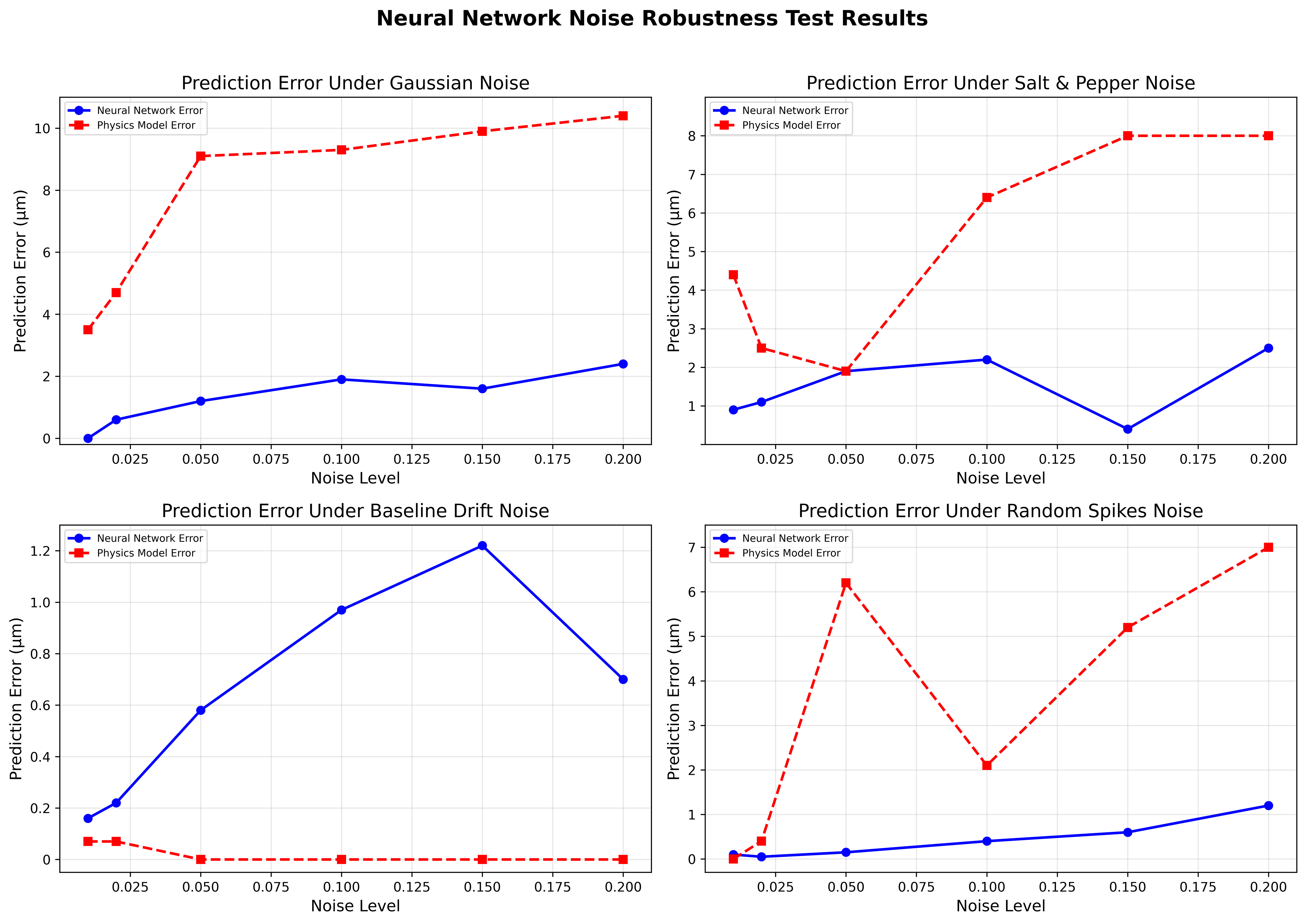
Figure 8. Comparison of prediction errors between AE-PINN and the physical model under different types and intensities of noise. AE-PINN: Attention-enhanced physics-informed neural network.
Table 5 summarizes the average errors for all noise levels. The average error of the AE-PINN across the four noise types was 0.962 μm, only 23.4% of the physical model’s average error of 4.119 μm. This corresponds to an error ratio (Physical/Neural) of 4.28, as shown in the last row of Table 5. This confirms the excellent noise robustness of the AE-PINN, stemming from the deep convolutional network’s ability to learn global spectral features rather than relying on local peaks, making it insensitive to local noise.
Quantitative comparison of noise robustness between AE-PINN and the physical model (averaged over all noise levels)
| Noise type | AE-PINN Avg.Error (μm) | Physical model Avg.Error (μm) | Error ratio (Physical/Neural) |
| Gaussian | 1.28 | 7.77 | 6.07 |
| Salt & pepper | 1.49 | 5.18 | 3.48 |
| Baseline drift | 0.64 | 0.027 | 0.04 |
| Random spikes | 0.44 | 3.5 | 7.95 |
| Average | 0.962 | 4.119 | 4.28 |
4.6. Verification of model continuous optimization via incremental learning
UAHIS integrates an incremental learning mechanism based on uncertainty Awareness: when a sample’s uncertainty exceeds the threshold τ, it triggers physical model verification, the sample, along with its physical model result, is stored in a “hard example buffer”. Periodically fine-tuning the AE-PINN with these samples can gradually improve the model performance for edge cases. Fine-tuning uses a “warm start” strategy with a learning rate of 10-4 for 10 epochs (hyperparameters given in Section 4.1).
The purpose of this incremental learning experiment is to validate the mechanism’s capability for continuous self-optimization. Accordingly, we intentionally conducted the experiment starting from the initial baseline AE-PINN model (RMSE = 1.4802 μm) rather than the complete model (RMSE = 1.1943 μm). This choice is deliberate: a baseline model with greater room for improvement provides a more rigorous and convincing test of the incremental learning mechanism, as any performance gain can be clearly attributed to the fine-tuning process, rather than being obscured by the diminishing returns typical of an already near-optimal model.
The 20 samples used for incremental learning were selected from the validation set based on their prediction errors. These selected samples will not participate in subsequent experiments after fine-tuning, and the rest of the validation samples are discarded after screening. The final model performance is evaluated exclusively on the held-out test set. Specifically, we computed the absolute error |d_pred - d_true| for each sample in the validation set and selected 20 samples with the largest errors. These samples represent the most challenging cases for the current model and are therefore the most informative for model fine-tuning. This selection strategy ensures that the incremental learning process focuses on the model’s weaknesses, maximizing improvement per additional training sample.
To validate this mechanism, we simulated the process by selecting 20 samples with the largest prediction errors from the validation set as challenging cases and used them to fine-tune the pre-trained model. The results are presented in Table 6. After fine-tuning, the RMSE on the entire test set decreased from 1.4802 to 1.3861 μm, a relative improvement of 6.36%; the MAE decreased from 1.1935 to 1.1215 μm; and the coefficient of determination R2 increased from 0.8580 to 0.8755. This demonstrates that fine-tuning with only 20 key samples can bring certain performance gains, confirming the feasibility of the incremental learning path.
Incremental learning performance improvement for AE-PINN
| Model state | RMSE (μm) | MAE (μm) | R2 | Relative improvement |
| AE-PINN (before fine-tuning) + incremental learning (after) | 1.4802 | 1.1935 | 0.858 | 6.36% |
| 1.3861 | 1.1215 | 0.8755 |
To further validate the effectiveness of the incremental learning strategy with different sample sizes, we conducted a gradient experiment comparing 10, 20, and 30 challenging samples. The RMSE decreased from 1.4802 μm (base model) to 1.4124 μm (10 samples, 4.58% improvement), 1.3861 μm (20 samples, 6.36% improvement), and 1.3717 μm (30 samples, 7.33% improvement) in the test set. The improvement increased with the number of samples while exhibiting diminishing returns, confirming that a small set of challenging samples (e.g., 20) is sufficient for effective model adaptation.
The core advantage of incremental learning is its targeted reinforcement of the model’s weaknesses, forming a virtuous cycle of “optimization-collection-re-optimization”. In the long run, the system can adaptively evolve to the optimal model state for its specific application scenario, transforming from a general model to a specialized expert.
5. CONCLUSION
This study proposes an UAHIS for SiC epilayer thickness measurement, integrating a physical benchmark model with an AE-PINN. A high-precision physical benchmark model based on multi-beam interference theory was established with corrected wavelength unit conversion, providing a reliable verification reference. The AE-PINN incorporates a channel attention mechanism and a spectral-consistency physical-constraint loss, achieving an RMSE of 1.194 μm in thickness prediction. The UAHIS uses Monte Carlo Dropout to quantify prediction uncertainty and implements adaptive switching between fast AE-PINN mode and physical model verification based on material-adaptive thresholds (SiC: 0.397 μm, Si: 0.252 μm). An uncertainty-Aware incremental learning mechanism enables continuous self-optimization using challenging samples encountered during measurements. For real data, the system achieved a mean absolute error of
DECLARATIONS
Authors’ contributions
Made substantial contributions to the conception and design of the study, as well as the methodology: Li, C.; Li, D.
Performed the software implementation, investigation, formal analysis, simulation experiments, and original draft writing and editing: Li, C.
Supervised the research and reviewed and edited the manuscript: Li, D.
Availability of data and materials
The datasets used and analyzed during the current study are available from the corresponding author upon reasonable request.
AI and AI-assisted tools statement
During the preparation of this manuscript, the AI tool DeepSeek (version V3.2-Exp, released 2026-02-16) was used exclusively for language-level editing. This tool was not involved in study design, data collection, data analysis, interpretation of results, or any core scientific content of this work. All authors take full responsibility for the accuracy, completeness, and final content of the manuscript.
Financial support and sponsorship
None.
Conflicts of interest
Both authors declared that there are no conflicts of interest.
Ethical approval and consent to participate
Not applicable.
Consent for publication
Not applicable.
Copyright
© The Author(s) 2026.
REFERENCES
1. Bagraev, N. T.; Kukushkin, S. A.; Osipov, A. V.; Ugolkov, V. L. Phase transitions in silicon-carbide epitaxial layers grown on a silicon substrate by the method of the coordinated substitution of atoms. Semiconductors 2022, 56, 321-4.
2. Costantini, J.; Guillaumet, M.; Lelong, G. Temperature-dependent optical absorption spectroscopy of ion irradiated silicon carbide epilayers on silicon. Appl. Phys. A. 2024, 130, 8025.
3. Bragin, A. V.; Pyanzin, D. V.; Sidorov, R. I.; Skvortsov, D. A. Recognition of dislocation structure of silicon carbide epitaxial layers by а neural network. Comput. Opt. 2020, 44, 653-9.
4. Mpilitos, C.; Amanatiadis, S.; Apostolidis, G.; Zygiridis, T.; Kantartzis, N.; Karagiannis, G. Development of a transmission line model for the thickness prediction of thin films via the infrared interference method. Technologies 2018, 6, 122.
5. Raissi, M.; Perdikaris, P.; Karniadakis, G. Physics-informed neural networks: a deep learning framework for solving forward and inverse problems involving nonlinear partial differential equations. J. Comput. Phys. 2019, 378, 686-707.
6. Li, G.; Ouyang, W.; Ouyang, W.; Liu, S. Static analysis of two-side supported 2-ply laminated glass panes through physics-informed neural networks. Eng. Struct. 2024, 309, 118038.
7. Wang, L.; Liu, G.; Wang, G.; Zhang, K. M‐PINN: a mesh‐based physics‐informed neural network for linear elastic problems in solid mechanics. Int. J. Numer. Methods. Eng. 2024, 125, e7444.
8. Ouyang, W.; Li, G.; Chen, L.; Liu, S. Physics‐informed neural networks for large deflection analysis of slender piles incorporating non‐differentiable soil‐structure interaction. Int. J. Numer. Anal. Methods. Geomech. 2024, 48, 1278-308.
9. Ye, X.; Ni, Y.; Ao, W. K.; Yuan, L. Modeling of the hysteretic behavior of nonlinear particle damping by Fourier neural network with transfer learning. Mech. Syst. Signal. Process. 2024, 208, 111006.
10. Peng, J.; Hua, Y.; Aubry, N.; Chen, Z.; Mei, M.; Wu, W. Data and physics-driven modeling for fluid flow with a physics-informed graph convolutional neural network. Ocean. Eng. 2024, 301, 117551.
11. Zhao, Y.; Li, D.; Wang, C.; Xi, H. An innovative end-to-end PINN-based solution for rapidly simulating homogeneous heat flow problems: an adaptive universal physics-guided auto-solver. Case. Stud. Therm. Eng. 2024, 56, 104277.
12. Cheng, C.; Zhang, G. Deep learning method based on physics informed neural network with resnet block for solving fluid flow problems. Water 2021, 13, 423.
13. Rui, E.; Chen, Z.; Ni, Y.; Yuan, L.; Zeng, G. Reconstruction of 3D flow field around a building model in wind tunnel: a novel physics-informed neural network framework adopting dynamic prioritization self-adaptive loss balance strategy. Eng. Appl. Comput. Fluid. Mech. 2023, 17, 2238849.
14. Jalili, D.; Jang, S.; Jadidi, M.; Giustini, G.; Keshmiri, A.; Mahmoudi, Y. Physics-informed neural networks for heat transfer prediction in two-phase flows. Int. J. Heat. Mass. Transf. 2024, 221, 125089.
15. Yadav, V.; Casel, M.; Ghani, A. RF-PINNs: reactive flow physics-informed neural networks for field reconstruction of laminar and turbulent flames using sparse data. J. Comput. Phys. 2025, 524, 113698.
16. Batuwatta-Gamage, C. P.; Rathnayaka, C.; Karunasena, H. C. P.; Jeong, H.; Karim, A.; Gu, Y. T. A novel physics-informed neural networks approach (PINN-MT) to solve mass transfer in plant cells during drying. Biosyst. Eng. 2023, 230, 219-41.
17. Oldenburg, J.; Borowski, F.; Schmitz, K.; Stiehm, M. Computation of flow through TAVI device by means of physics informed neural networks. Curr. Dir. Biomed. Eng. 2022, 8, 741-4.
18. Ma, Y.; Xu, X.; Yan, S.; Ren, Z. A preliminary study on the resolution of electro-thermal multi-physics coupling problem using physics-informed neural network (PINN). Algorithms 2022, 15, 53.
19. Wang, Y.; Fan, Q.; Dai, F.; Wang, R.; Ding, B. A physics-data-driven method for predicting surface and building settlement induced by tunnel construction. Comput. Geotech. 2025, 179, 107020.
20. Chen, S.; Ji, X.; Shao, H.; Zhang, Y. A physics-informed traffic state estimation model for freeways under sparse observation data. Transportmetrica. B. 2025, 13, 2564701.
21. Ren, P.; Rao, C.; Liu, Y.; Wang, J.; Sun, H. PhyCRNet: physics-informed convolutional-recurrent network for solving spatiotemporal PDEs. Comput. Methods. Appl. Mech. Eng. 2022, 389, 114399.
22. Markidis, S. The old and the new: can physics-informed deep-learning replace traditional linear solvers? Front. Big. Data. 2021, 4, 669097.
23. Wu, G.; Fang, Y.; Wang, Y.; Wu, G.; Dai, C. Predicting the dynamic process and model parameters of the vector optical solitons in birefringent fibers via the modified PINN. Chaos. Solitons. Fractals. 2021, 152, 111393.
24. Bai, X.; Wang, Y.; Zhang, W. Applying physics informed neural network for flow data assimilation. J. Hydrodyn. 2020, 32, 1050-8.
25. Jagtap, A. D.; Karniadakis, G. E. Extended physics-informed neural networks (XPINNs): a generalized space-time domain decomposition based deep learning framework for nonlinear partial differential equations. Commun. Comput. Phys. 2025, 28, 2002-41.
26. Mehta, P. P.; Pang, G.; Song, F.; Karniadakis, G. E. Discovering a universal variable-order fractional model for turbulent Couette flow using a physics-informed neural network. Fract. Calc. Appl. Anal. 2019, 22, 1675-88.
27. Qian, Y.; Zhang, Y.; Huang, Y.; Dong, S. Physics-informed neural networks for approximating dynamic (hyperbolic) PDEs of second order in time: Error analysis and algorithms. J. Comput. Phys. 2023, 495, 112527.
28. Qian, Y.; Zhang, Y.; Dong, S. Error analysis and numerical algorithm for PDE approximation with hidden-layer concatenated physics informed neural networks. J. Comput. Phys. 2025, 530, 113906.
29. Liu, D.; Liu, Y.; Dang, H.; et al. The neutron transport equation in exact differential form. Sci. China. Phys. Mech. Astron. 2025, 68, 2642.
30. Son, H.; Lee, M. A PINN approach for identifying governing parameters of noisy thermoacoustic systems. J. Fluid. Mech. 2024, 984, A21.
31. Yan, S.; Chen, Y.; Cao, W.; Li, H. Enhancing U-Net with low-rank attention skip block for 3D point cloud segmentation. Neurocomputing 2025, 626, 129593.
32. Cao, X.; Chen, Y.; Cao, W. Proximal PanNet: a model-based deep network for pansharpening. AAAI. Conf. Artif. Intell. 2022, 36, 176-84.
Cite This Article
 Open Access
How to Cite
Download Citation
Export Citation File:
Type of Import
Tips on Downloading Citation
Citation Manager File Format
Type of Import
Direct Import: When the Direct Import option is selected (the default state), a dialogue box will give you the option to Save or Open the downloaded citation data. Choosing Open will either launch your citation manager or give you a choice of applications with which to use the metadata. The Save option saves the file locally for later use.
Indirect Import: When the Indirect Import option is selected, the metadata is displayed and may be copied and pasted as needed.
About This Article
Copyright

Data & Comments
Data
0










Comments
Comments must be written in English. Spam, offensive content, impersonation, and private information will not be permitted. If any comment is reported and identified as inappropriate content by OAE staff, the comment will be removed without notice. If you have any queries or need any help, please contact us at [email protected].