

Disturbance-aware collaborative routing for concurrent emergency response
 0
0 
Abstract
Concurrent emergency response (CER) scenarios pose significant challenges to emergency vehicle (EV) routing and scheduling due to dynamic traffic disturbances and resource competition. Existing methods typically decouple routing and scheduling and fail to capture disturbance-aware traffic dynamics, leading to suboptimal performance. This paper proposes a disturbance-aware hierarchical framework that jointly optimizes route generation and collaborative scheduling. A Disturbance-Aware Graph WaveNet (DAGWN) is developed to model spatiotemporal traffic evolution and predict traffic states and disturbance intensity. Building on this, a unified scheduling cost model incorporating task urgency, travel time, route conflict, and fairness is formulated and solved via a minimum cost flow (MCF) approach. Experiments on a SUMO-based urban traffic simulation demonstrate that the proposed method improves prediction accuracy and reduces total completion time, average response time, and maximum response time compared with state-of-the-art baselines. The results validate the effectiveness of integrating disturbance-aware modeling with joint routing and scheduling for efficient emergency response.
Keywords
INTRODUCTION
With rapid urbanization and continuous population growth, emergency incidents have become more frequent, threatening residents’ lives, property, and urban stability. According to the national emergency and rescue statistics released by the Fire and Disaster Management Agency of Japan, emergency dispatches in Japan reached 7,720,740 in 2024, about 1.0% higher than the previous year[1]. The increasing demand for emergency services has imposed sustained pressure on urban emergency response systems.
Emergency Response Time (ERT), defined as the interval between receiving an emergency call and the arrival of emergency vehicles (EVs) at the incident scene, is a key indicator of emergency response performance[2]. Medical and emergency management studies show that delayed emergency response may significantly reduce rescue effectiveness and survival probability[3,4]. Accordingly, reducing ERT and ensuring timely arrival are central objectives in Emergency Management System (EMS) design and optimization[5].
Various route planning strategies have been proposed to reduce ERT by shortening EV travel time[6-8]. Nevertheless, most existing methods minimize travel time and are mainly designed for single-vehicle routing of social vehicles (SVs). In Concurrent emergency response (CER) scenarios, shorter travel time does not necessarily imply better response efficiency, because route quality should be evaluated by the overall response outcome rather than individual vehicle efficiency. Optimizing only travel time may ignore task heterogeneity, resource competition, and multi-EV coordination, thereby producing routing decisions that are inconsistent with system-level emergency response objectives. Therefore, EV routing and scheduling in CER scenarios still face the following challenges.
Existing traffic prediction methods are typically trained under regular traffic conditions, making it difficult to capture incident-induced disturbances and their propagation across the road network. As a result, they may fail to reflect route risk and traffic capacity degradation. On the other hand, multiple EVs operating simultaneously compete for limited vehicle and road resources. When they travel to nearby incident areas or pass through the same bottleneck segments, route overlaps, local congestion, and mutual interference may occur, reducing overall response efficiency.
Existing studies also commonly decouple route planning from task scheduling, although they are tightly coupled in CER scenarios. Route selection directly affects response time, road resource usage, and vehicle availability for subsequent tasks, while scheduling decisions can in turn change route feasibility and congestion risk. This suggests that traffic prediction alone is insufficient if it only describes future traffic states. Its results should be transformed into route decision information to support the evaluation of route risk, capacity degradation, and potential route conflicts. In this way, traffic prediction, candidate route generation, and collaborative scheduling form an integrated decision process, thereby improving overall emergency response efficiency in CER scenarios.
In summary, CER is affected by dynamic traffic evolution, incident disturbance propagation, and competition for limited emergency resources. Traditional methods typically rely on sequential optimization with fixed routes or task assignments, which may achieve local optimization but cannot ensure global coordination in multi-vehicle and multi-task scenarios. Accordingly, coordinated optimization of EV route selection and task scheduling under dynamic traffic and concurrent tasks remains an open problem. To address these challenges, this paper proposes a disturbance-aware routing and collaborative scheduling method for CER, integrating traffic prediction, route generation, and task scheduling into a unified optimization process. By modeling incident disturbance propagation across the road network, the proposed method transforms prediction results into decision information for candidate route generation and vehicle-task assignment, enabling consistent routing and scheduling decisions and improving the overall response efficiency of multiple emergency tasks.
The main contributions of this paper are summarized as follows:
• We formulate CER as a coupled route-task-vehicle optimization problem under disturbance-aware dynamic traffic evolution, enabling a hierarchical framework that integrates traffic prediction, candidate route generation, and collaborative scheduling.
• We extend Graph WaveNet with incident-induced disturbance propagation modeling and a dual-head output structure to simultaneously predict future traffic states and segment-level disturbance intensity, thereby supporting decision-oriented emergency route generation.
• We design a unified urgency-aware scheduling cost that integrates response efficiency, route conflict, and fairness under concurrent emergency resource competition, where a nonlinear urgency weight, route conflict penalty, and logarithmic fairness compensation are introduced to support stable multi-task scheduling.
• Extensive experiments demonstrate that disturbance-aware route generation mainly improves robustness under high-disturbance conditions, while collaborative scheduling significantly reduces worst-case response delays, thereby improving overall CER efficiency.
Related work
Emergency vehicle routing and priority control
Emergency vehicle routing and priority control have been widely studied to reduce response time under dynamic urban traffic conditions. Existing studies improve EV passage mainly through real-time route adjustment, intersection signal preemption, and cooperative yielding for surrounding social vehicles[6-13]. These methods show that EV mobility can be enhanced by adapting routes, reserving intersection capacity, and coordinating nearby traffic participants.
However, their decision scope remains largely local. Dynamic routing optimizes a given EV route using segment-level congestion or travel-time costs, while signal preemption and yielding strategies reduce delays at specific intersections or local areas. In CER scenarios, such local decisions may increase route conflicts or delay other urgent tasks because multiple tasks and EVs compete for feasible routes and response resources. This motivates coupling EV routing with collaborative scheduling, so that candidate routes can be evaluated from a system-level perspective under concurrent incidents and resource competition.
Disturbance-aware traffic prediction
Recent traffic prediction studies use graph neural networks and Transformer-based architectures to capture spatiotemporal dependencies in urban road networks[14-18]. They improve modeling of road-network diffusion, temporal evolution, adaptive spatial correlations, and long-range spatiotemporal patterns. However, most models target regular traffic conditions and rely mainly on historical patterns, making them insufficient for modeling incident-induced capacity degradation and disturbance propagation across neighboring or downstream segments.
Some studies have incorporated event or incident information into traffic prediction, showing that abnormal events affect future traffic states and spatial dependencies[19,20]. Nevertheless, they still focus mainly on prediction accuracy, and the predicted incident impact is rarely converted into route-level decision information for emergency response. In CER scenarios, traffic prediction should provide both future traffic states and disturbance-aware information to support candidate route generation and collaborative scheduling.
Emergency scheduling
Emergency scheduling studies have shifted from isolated dispatching to joint dispatching, relocation, and multi-period resource redistribution under uncertain and time-varying demand[21-23]. These studies improve emergency resource availability and responsiveness, but they mainly focus on vehicle deployment or assignment rather than the joint evaluation of task urgency, route quality, and resource competition under concurrent incidents.
Another research line formulates emergency response as multi-vehicle multi-task allocation, path planning, or matching-based optimization[24-28]. These formulations provide useful structures for assigning limited emergency resources to multiple demands. Such methods still treat route information as fixed input or evaluate assignment costs mainly by distance, travel time, or matching feasibility. Accordingly, collaborative scheduling requires a unified formulation that integrates dynamic traffic disturbances, concurrent tasks, and limited emergency resources.
EXPERIMENTAL
This section presents the proposed disturbance-aware routing and collaborative scheduling framework. As illustrated in Figure 1, the framework contains two coupled layers: the lower layer predicts disturbance-aware traffic states and generates candidate routes, while the upper layer jointly optimizes EV-task assignment and route selection under task urgency and resource constraints. This design integrates traffic perception and collaborative scheduling into a unified decision-making process. Although the two layers are coupled through candidate routes and route-level decision information, they are designed in a modular manner rather than as a fully end-to-end pipeline. The lower layer provides a set of feasible candidate routes and their disturbance-aware travel information, while the upper layer requires only these route-level inputs to construct task-EV-route triplets and perform collaborative scheduling. Therefore, the upper-layer MCF scheduler is not structurally tied to a specific traffic prediction model or route generation method. Even when the lower-layer predictor is replaced by static shortest-path routing or another routing module, the upper-layer scheduling formulation remains applicable. This design limits the direct dependence of the scheduling layer on a particular prediction model, while still allowing disturbance-aware prediction to improve the quality of candidate routes.
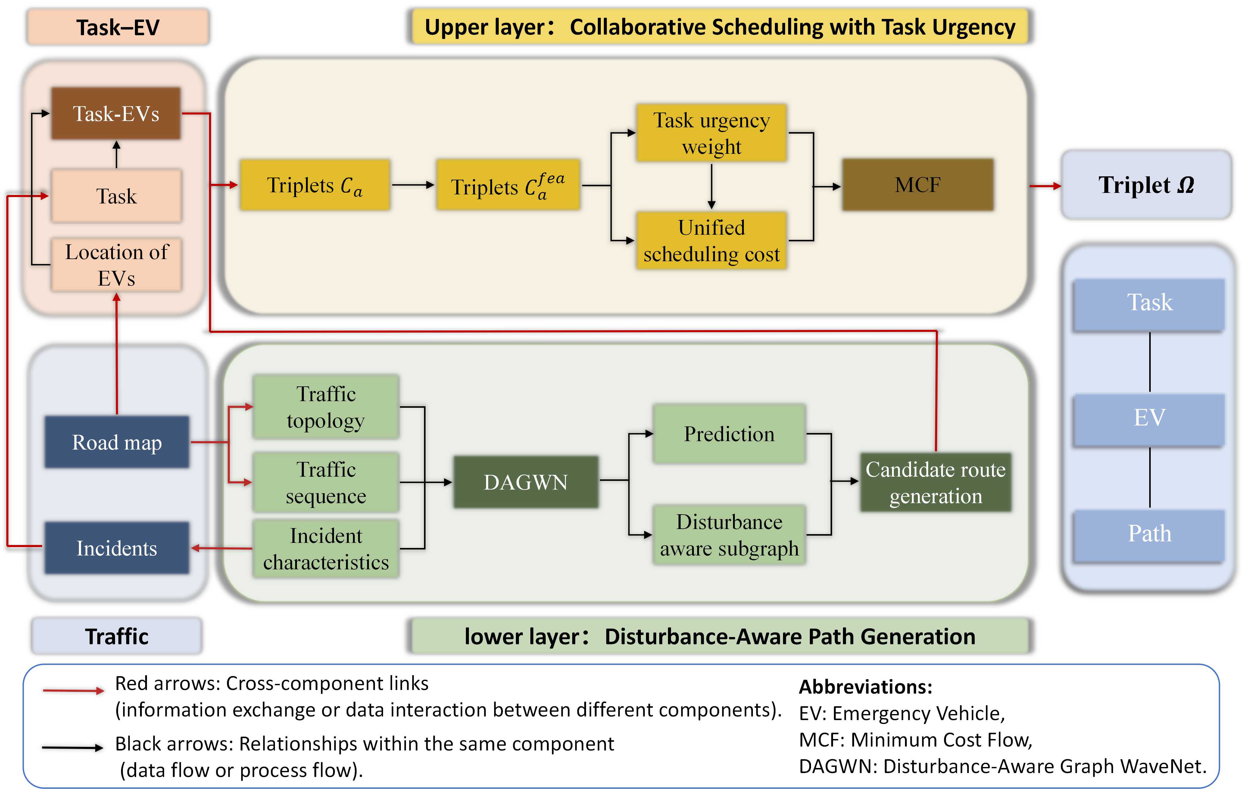
Figure 1. Overall framework of the proposed method.
Problem formulation
The road network is modeled as a directed graph G = (
Incident impacts are further incorporated into traffic modeling. Let
The incidents are then mapped to response tasks R = {r1, r2, …, r|R|}, where each task corresponds to an incident to be handled. For each task ri
Based on the above task, EV, and route definitions, let xijn denote whether evj
subject to:
These constraints ensure that each task is served by at least one feasible EV, each available EV is assigned to at most one task within a scheduling period, and only feasible routes that start from the assigned EV’s current location and satisfy reachability constraints can be selected.
Disturbance-aware route generation
The lower layer uses DAGWN to characterize incident-affected traffic evolution for route generation. DAGWN combines three adjacency supports: the physical adjacency matrix for direct road connectivity, the adaptive adjacency matrix for latent traffic correlations, and the disturbance-aware adjacency matrix for incident-induced spatial propagation. These supports collectively model traffic states and disturbance intensity.
Incident disturbance modeling
Incidents are treated as external disturbance sources whose impacts diffuse along the road network to downstream areas. For each incident s, the shortest hop distance from
Here, the first three components represent source membership, normalized topological distance, and distance-based decay, where ω > 0 controls the decay rate. In this study, ω is set as a fixed global hyperparameter. For segments beyond the maximum propagation range, the disturbance value is set to zero. The incident severity is
When multiple incidents occur, their disturbance features are stacked into a disturbance tensor
Disturbance-aware Graph WaveNet
DAGWN is built upon Graph WaveNet[16] and integrates temporal modeling with incident spatial diffusion to predict traffic capacity and disturbance intensity for route generation. Figure 2 shows the overall architecture of DAGWN.
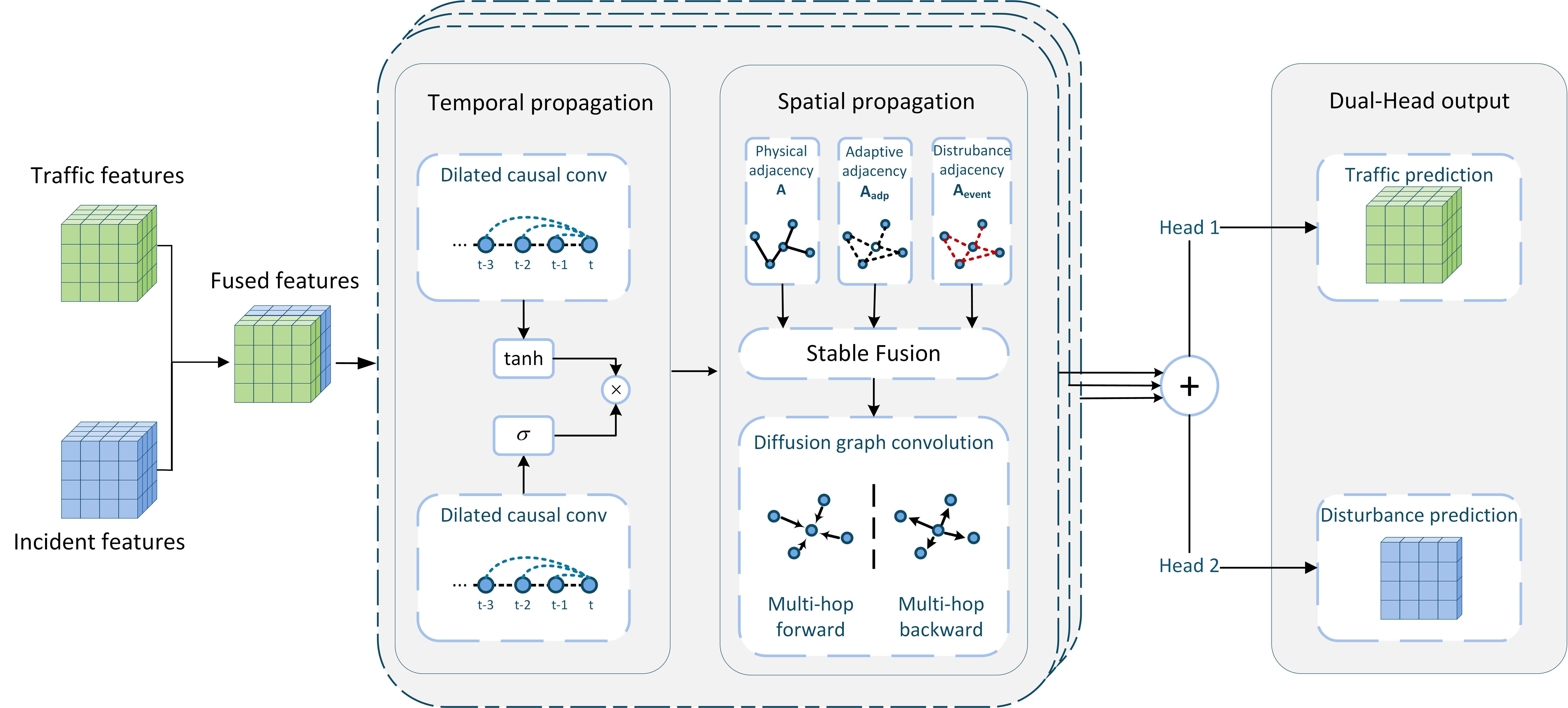
Figure 2. Disturbance-aware Graph WaveNet framework.
A. Graph convolution layer
For spatial modeling, DAGWN uses diffusion graph convolution to describe traffic feature propagation on a directed graph. Let
where K is the diffusion order, and Wk1 and Wk2 are learnable parameters for forward and backward diffusion, respectively[16].
A single adjacency matrix still cannot simultaneously capture network topology, latent segment correlations, and incident-induced disturbance relationships. Accordingly, diffusion graph convolution is extended with multiple supports
In the support set, the physical adjacency matrix A represents actual road connectivity, while the adaptive adjacency matrix
where H1 and H2 denote embeddings of source and target segments[16].
To model local incident propagation, the disturbance-aware adjacency matrix Aevent is constructed. For each segment ei, its disturbance intensity is computed from
The disturbance relationship between two segments is then expressed as
To prevent disturbance information from dominating spatial dependency modeling, a stabilization mechanism reweighs the disturbance-aware adjacency matrix and fuses it with the adaptive adjacency matrix through a residual connection.
where λe and μa denote the disturbance adjacency weight and residual fusion coefficient, respectively. The three adjacency supports are designed to capture complementary spatial dependencies: the physical adjacency preserves road-topology constraints, the adaptive adjacency captures latent traffic correlations beyond direct connectivity, and the disturbance-aware adjacency emphasizes incident-induced local propagation. The residual fusion is therefore used as a stable and lightweight mechanism to retain general traffic correlations while preventing sparse disturbance signals from excessively dominating spatial dependency learning. Based on the fused supports, graph convolution is written as
where
B. Temporal convolution layer
To capture the temporal evolution of incident-affected traffic states, DAGWN uses dilated causal convolution for temporal feature extraction.
Let the input tensor be
Temporal dependencies are modeled by gated dilated convolution:
where
For a one-dimensional temporal sequence of a single channel, dilated causal convolution is written as
where Kt denotes the temporal kernel size, and fτ denotes the kernel parameter at position τ. When δ > 1, sparse temporal sampling enlarges the receptive field without significantly increasing the parameter size[16].
C. Dual-head output structure with disturbance awareness
In the output layer, DAGWN adopts a dual-head structure to separately predict traffic states and estimate incident impacts. Since incident disturbances are local and sparse, a single traffic-state regression head may suppress them or treat them as noise, weakening the model’s ability to describe the affected range and intensity. To address this issue, two output heads are introduced to preserve both global traffic evolution and local disturbance effects. The primary head (head-1) predicts future traffic states for route generation, while the disturbance-aware subgraph head (head-2) estimates segment-level disturbance intensity
During training, the two heads are jointly optimized with the following overall loss:
where Lossreg and Lossmask are the losses of head-1 and head-2, respectively, and λ1 is the weighting coefficient.
Dynamic weight update-based candidate route generation
Under incident-affected traffic states, static edge weights based on length or average travel time cannot reflect local capacity degradation. As a result, Dijkstra edge weights are dynamically updated using predicted travel time and disturbance intensity. The cost of segment e is defined as coste = te + λ2g(e), where te is its predicted travel time and λ2 is the disturbance intensity weight. To provide multiple feasible choices for upper-level scheduling, key segments in the current optimal route are penalized after each search to guide subsequent searches toward more diverse and less locally similar alternatives.
Thus, traditional Dijkstra-based routing is extended to dynamic multi-candidate route construction for complex emergency traffic environments.
Collaborative scheduling with task urgency
After candidate routes are generated, scheduling in concurrent emergency scenarios is formulated as a Multi-Vehicle Multi-Task Allocation (MVMTA) combinatorial optimization problem, where task-EV-route combinations must be selected under time constraints, resource limitations, and task competition. The combinatorial explosion among tasks, vehicles, and routes makes the problem NP-hard[4], making direct enumeration and conventional methods difficult to apply in complex settings. To solve this problem, task assignment and route selection are unified through task-EV-route triplets, which transform scheduling into a discrete combinatorial decision process. Infeasible combinations are pruned to form the feasible solution set, and a two-stage scheduling cost function combining task urgency and route cost is used to determine the final decision through unified optimization.
Decision unit construction and feasibility screening
Tasks, EVs, and routes are modeled as triplet decision units
Since Ca may contain infeasible triplets, evaluating all candidates can introduce invalid solutions and increase computational complexity. To avoid this, feasibility screening is applied before optimization. First, type matching is checked to ensure that the EV assigned to each task belongs to the required vehicle type set of that task. Second, route feasibility is verified by removing routes with closed or inaccessible road segments. Third, explicitly invalid triplets caused by routing failure, task invalidation, or unavailable EVs are excluded. After filtering, Ca is reduced to a feasible set
Unified scheduling cost with task urgency
After feasibility screening, each triplet (i, j, n) represents an executable scheduling scheme. The scheduling objective is to balance task urgency and execution cost under limited resources, so high-urgency tasks should be prioritized without sacrificing overall system efficiency. Accordingly, task priority weights are first constructed to characterize task importance, and a unified scheduling cost function is then defined to integrate task urgency and route execution cost.
D. Task urgency weight
To prevent high-risk tasks from being delayed by schemes that minimize only route length or travel time, a task-urgency weight is introduced into the scheduling cost function. For each task i, the estimated arrival times of all feasible schemes are denoted as
In emergency response, delay has nonlinear and task-dependent effects. A task with a high emergency level, high waiting risk, and strong worst-case delay pressure should receive sharply increased priority because additional delay may cause more serious consequences. Accordingly, the task urgency weight is defined in exponential form to amplify the combined high-risk factors:
Where αu, αh, and αv control the contributions of the three factors, and ui denotes the urgency of ri obtained from the task level.
The life risk term hi reflects the potential loss caused by waiting time under current traffic and resource conditions and adapts the nonlinear risk definition in[29] to CER scheduling.
where λ balances base waiting risk and additional delay risk, μ controls the increase rate after the response baseline is exceeded, and [x]+ = max(x, 0). The first term measures the base risk associated with the minimum achievable arrival time, while the second term is activated only when this time exceeds
The relative time pressure under the worst response condition is defined as
where
E. Unified scheduling cost
For each feasible triplet (i, j, n), the scheduling cost evaluates the global benefit of assigning EV evj to task ri via route
Here,
The time cost is computed as
where
The conflict cost consists of route load and overlap risk:
The load risk is defined as
where
For a feasible triplet
where route similarity is computed by the Jaccard index to measure the relative proportion of shared road segments and avoid overestimating conflicts on longer routes.
The fairness compensation term is defined as
Since
Minimum cost flow-based collaborative scheduling
After the unified scheduling cost is computed, the scheduling problem is formulated as a Minimum Cost Flow (MCF) problem, which is suitable for CER scheduling because it optimizes additive costs under capacity constraints and enables global coordination of multiple task-EV-route decisions with limited resources. A directed flow network is constructed to match tasks, EVs, and candidate routes, where edge costs are defined by
RESULTS AND DISCUSSION
Experimental setup and scenario design
The proposed method is implemented in Python 3.10 with SUMO 1.18.0 on an OpenStreetMap road network of Shinjuku, Tokyo, which contains 3,736 nodes and 8,466 edges. To emulate high-density urban emergency conditions, peak-hour traffic is generated at 1 s intervals over a simulation horizon of 2,400 s. All experiments are run on a NVIDIA GeForce RTX 4090 GPU with 24 GB memory.
To reproduce CER conditions with concurrent emergency demands, three simultaneous incidents occur in each scenario at the simulation time of t = 900 s, with heterogeneous types, severities, locations, and occurrence probabilities defined in Table 1. EVs are deployed according to representative facilities in Shinjuku, including 14 ambulances from four hospitals, 7 fire engines from two fire stations, and 7 police vehicles from two police stations. Traffic states are updated every 60 s to capture the temporal evolution of disturbance propagation and network congestion. For the lower-layer prediction task, each scenario generates a pair of baseline and disturbance samples. The baseline sample is obtained from an incident-free simulation under the same road network, traffic demand, signal settings, and simulation horizon, while the disturbance sample is generated by introducing the corresponding incidents into the same simulation setting. The paired samples are used to compute the disturbance intensity labels for training the disturbance-aware head.
Incident type and distribution settings
| Type | Total | Severity | Location | ||||||
| 1 | 2 | 3 | 4 | 5 | Mid | Up | Down | ||
| Single | 0.20 | 0.7 | 0.3 | 0 | 0 | 0 | 0.8 | 0.1 | 0.1 |
| Collision | 0.35 | 0 | 0.6 | 0.4 | 0 | 0 | 0.2 | 0.4 | 0.4 |
| Crash | 0.10 | 0 | 0 | 0.5 | 0.3 | 0.2 | 0.5 | 0.25 | 0.25 |
| Fire | 0.05 | 0 | 0 | 0.5 | 0.3 | 0.2 | 0.5 | 0.25 | 0.25 |
| Explosion | 0.05 | 0 | 0 | 0 | 0.3 | 0.7 | 0.7 | 0.15 | 0.15 |
| Public | 0.05 | 0 | 0.4 | 0.4 | 0.2 | 0 | 0.3 | 0.4 | 0.3 |
| Infrastructure | 0.15 | 0.6 | 0.3 | 0.1 | 0 | 0 | 0.3 | 0.5 | 0.2 |
| Disasters | 0.05 | 0 | 0.4 | 0.3 | 0.2 | 0.1 | 0.5 | 0.25 | 0.25 |
The experimental scenarios are designed to represent high-density urban CER conditions with simultaneous incidents and resource competition, rather than infeasible extreme cases where all access routes to an incident are completely blocked. In such fully disconnected cases, the problem becomes one of emergency accessibility restoration rather than route-scheduling optimization.
Disturbance-aware traffic prediction evaluation
Implementation details
In DAGWN, the model is trained for 500 epochs using Adam with a learning rate of 0.001, and its loss combines Mean Squared Error for future-state prediction and Smooth L1 Loss for disturbance prediction with adaptive weighting via learnable uncertainty parameters.
To improve the reproducibility of the experiments, the key experimental parameters used in the disturbance-aware traffic prediction evaluation are summarized in Table 2.
Key implementation and experimental parameters
| Symbol | Parameter name | Value |
| t | Incident occurrence time | 900 s |
| T | Historical window length | 10 steps (10 min) |
| H | Prediction horizon | 10 steps (10 min) |
| F | Feature dimension per segment and time step | 5 |
| O | Number of hidden channels (hidden dimension) | 64 |
| K | Diffusion order | 2 |
| dmax | Maximum propagation range | 10 hops |
| ω | Disturbance decay rate | 2.0 |
| λe | Disturbance adjacency weight | 0.5 |
| μa | Residual fusion coefficient | 0.1 |
| B | Batch size | 4 |
| λ1 | Weighting coefficient of the disturbance loss | 0.5 |
| λ2 | Disturbance intensity weight | 1.0 |
Baseline methods
Five representative spatiotemporal forecasting models are adopted as baselines to evaluate the effectiveness of disturbance-aware propagation modeling under incident-affected traffic conditions. These baselines include Diffusion Convolutional Recurrent Neural Network (DCRNN)[14], Spatio-Temporal Graph Convolutional Network (STGCN)[15], Graph WaveNet (GWN)[16], DGCRN[17], and Spatio-Temporal Adaptive Embedding Transformer (STAEformer)[18].
Evaluation metrics
The prediction performance is evaluated using the following metrics.
• Mean-based error metrics: Mean Squared Error (MSE), Mean Absolute Error (MAE), and Root Mean Squared Error (RMSE) evaluate overall prediction errors from different perspectives. MSE emphasizes large deviations, MAE measures average absolute deviation, and RMSE reports squared-error-based deviation in the original data scale.
• Percentile-based error metrics: P50, P90, and P99 represent the 50th, 90th, and 99th percentiles of absolute errors, reflecting typical prediction performance, high-error cases, and tail robustness, respectively.
Results and analysis
Figure 3 and Table 3 demonstrate that DAGWN achieves the best performance in terms of Loss, MSE, and RMSE under incident-affected traffic conditions, while obtaining the second-best MAE result. Although DAGWN and GWN both reduce errors rapidly and converge in fewer epochs, DAGWN maintains a lower and more stable curve in the later training stages. These results indicate that explicitly modeling disturbance propagation significantly improves the ability to capture abnormal traffic evolution.The similar trends in Figure 3A, B and D are expected. In this figure, the plotted loss is the MSE-based prediction loss used to monitor model convergence, so the Loss curve in Figure 3A is naturally close to the MSE curve in Figure 3B. In addition, RMSE is computed as the square root of MSE; therefore, Figure 3D preserves the same variation trend as Figure 3B, while the value range is compressed after the square-root transformation. These relationships explain why the Loss, MSE, and RMSE curves show highly similar convergence patterns.
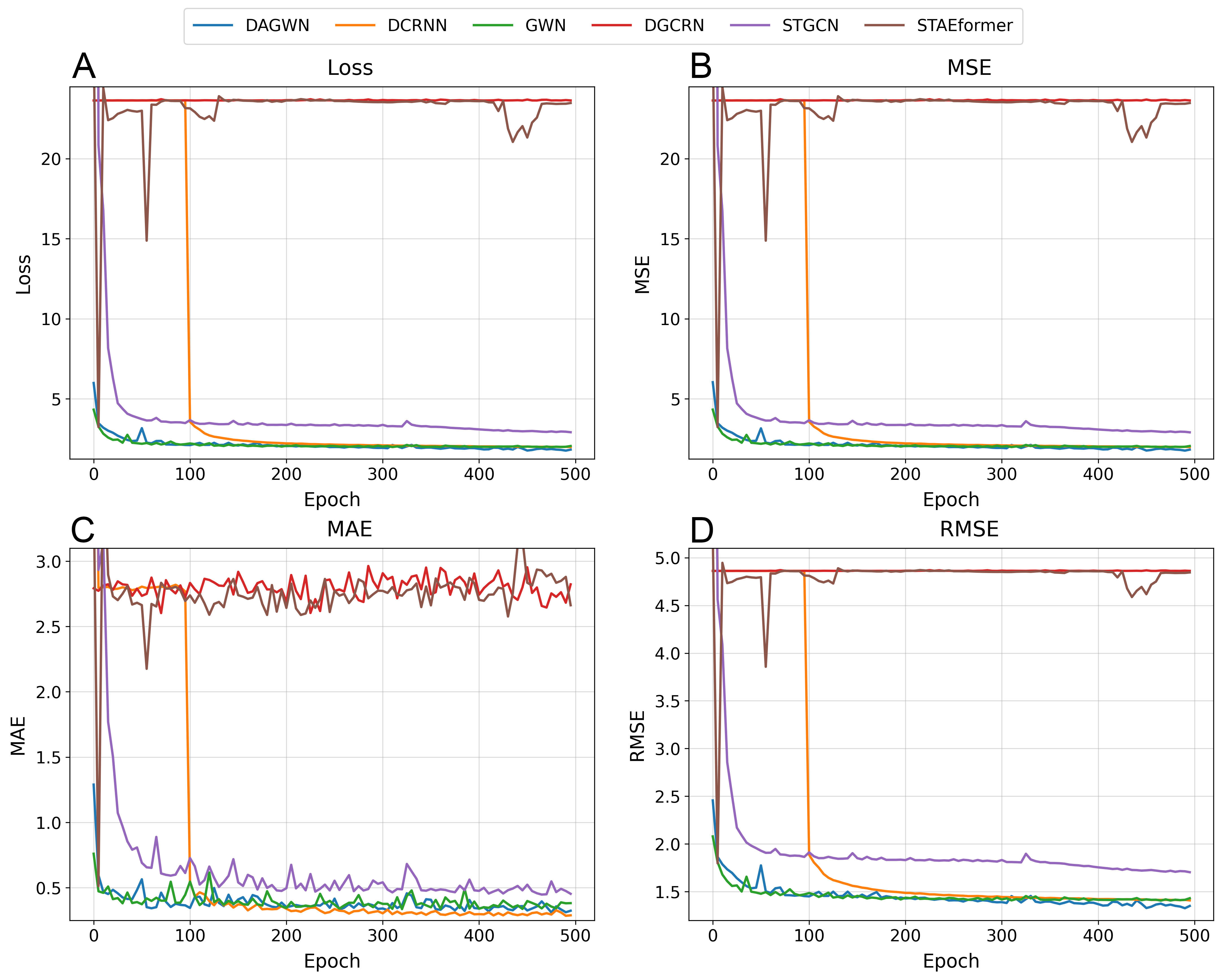
Figure 3. Training curves of different traffic prediction models over 500 epochs in terms of (A) training loss; (B) mean squared error (MSE); (C) mean absolute error (MAE); and (D) root mean squared error (RMSE). DAGWN: Disturbance-Aware Graph WaveNet; GWN: Graph WaveNet; DCRNN: Diffusion Convolutional Recurrent Neural Network; DGCRN: Dynamic Graph Convolutional Recurrent Network; STGCN: Spatio-Temporal Graph Convolutional Network; STAEformer: Spatio-Temporal Adaptive Embedding Transformer.
Performance comparison of different models
| Algorithm | Loss | MSE | MAE | RMSE |
| DAGWN | 1.824621 | 1.824525 | 0.323446 | 1.350750 |
| DCRNN | 1.984230 | 1.984181 | 0.288422 | 1.408610 |
| GWN | 2.049012 | 2.048991 | 0.381609 | 1.431430 |
| STGCN | 2.909792 | 2.904125 | 0.453034 | 1.704149 |
| STAEformer | 23.475807 | 23.475746 | 2.662695 | 4.845178 |
| DGCRN | 23.636180 | 23.635237 | 2.822613 | 4.861609 |
DCRNN also converges, but its training loss remains relatively high in the early stage and decreases notably after about 100 epochs, indicating slower convergence and lower stability than DAGWN. Although DCRNN achieves the lowest MAE, its weaker squared-error metrics indicate lower robustness to large deviations. STGCN converges at a higher error level than DAGWN, GWN, and DCRNN, suggesting that fixed graph convolution is less adaptive to dynamic spatial dependencies under incident disturbances. DGCRN and STAEformer maintain high training errors throughout training, suggesting limited ability to fit disturbed traffic states.
As shown in Figure 4, the performance gap among different models becomes substantially larger at P90 and P99, indicating that disturbance-aware modeling mainly improves robustness under high-impact traffic perturbations rather than regular traffic conditions. DAGWN achieves the best P99 value of 6.67 and the second-best P50 and P90 values of 0.072 and 0.40, respectively, showing stronger control of extreme errors and better robustness to incident-induced traffic variations. In contrast, DGCRN and STAEformer perform acceptably at P50 but deteriorate sharply at higher quantiles, indicating weak tail-error control and suggesting that these models fail to capture the spatial diffusion and temporal persistence of incident-induced disturbances.
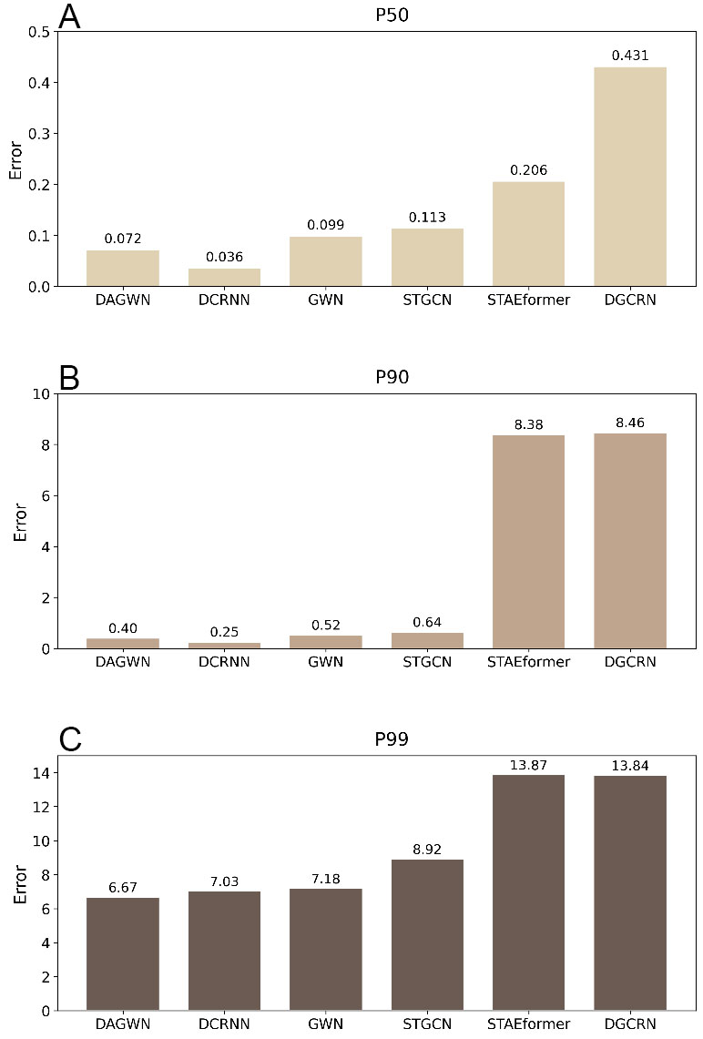
Figure 4. Error distribution comparison (P50, P90, P99) across different models. (A) comparison of the median absolute prediction error (P50); (B) comparison of the 90th-percentile absolute prediction error (P90); and (C) comparison of the 99th-percentile absolute prediction error (P99). DAGWN: Disturbance-Aware Graph WaveNet; DCRNN: Diffusion Convolutional Recurrent Neural Network; GWN: Graph WaveNet; STGCN: Spatio-Temporal Graph Convolutional Network; STGCN: Spatio-Temporal Graph Convolutional Network; DGCRN: Dynamic Graph Convolutional Recurrent Network.
Collaborative scheduling performance evaluation
Implementation details
In the task urgency weight, αu, αh, and αv are set to 0.5, 0.3, and 0.2, respectively, making the task level the dominant factor while using life risk and relative time pressure as supplementary risk information. For the life risk term, λ = 0.4 balances base risk and additional delay risk, while μ = 2 controls the growth rate after the response baseline is exceeded. The relative delay coefficient β = 0.5 treats relative delay as an auxiliary penalty while keeping absolute response time as the main objective. All reported results are averaged over 200 simulation runs.
The key parameters in the proposed framework have different functional roles across the prediction, route generation, and scheduling layers. The disturbance decay parameter controls the spatial range of incident influence: a larger value leads to wider propagation, whereas a smaller value makes the disturbance more localized. The adjacency fusion weights balance incident-induced propagation and general traffic correlations, preventing the disturbance-aware adjacency from dominating spatial dependency modeling. The disturbance penalty in candidate route generation adjusts the trade-off between travel-time minimization and avoidance of highly disturbed segments. In the upper-layer scheduling cost, the urgency-weight coefficients determine the relative importance of task level, life risk, and time pressure, while the relative delay coefficient controls the penalty for selecting routes that deviate from the best feasible response time. These parameters were selected to maintain the primary role of response efficiency while allowing disturbance risk, route conflict, and fairness to influence the final scheduling decision.
Baseline methods
Since the MVMTA problem is NP-hard, representative heuristic, matching-based, and evolutionary baselines are adopted for comparison, including Random, Greedy, Nearest Neighbor, Hungarian, Multiobjective Evolutionary Algorithm Based on Decomposition Using Simulated Annealing (G-MOEA/D-SA)[21], and Non-dominated Sorting Genetic Algorithm II for the Integrated Emergency Vehicle Scheduling Model (NSGA-II-IEV)[25].
Evaluation metrics
Scheduling performance under concurrent emergency scenarios is evaluated from three aspects: overall efficiency, worst-case performance, and critical task responsiveness:
• Overall efficiency: Actual completion time measures the time required to complete all tasks, while average response time reflects the mean response delay across tasks.
• Worst-case performance: Maximum response time captures the largest task delay and reflects scheduling robustness.
• Critical task responsiveness: Average response time of high-priority tasks evaluates whether critical tasks are prioritized effectively.
Performance analysis
As shown in Figure 5, MCF achieves the best results across all three overall metrics. Specifically, Figure 5A-C present the total completion time, average response time, and maximum response time, respectively. This demonstrates that the proposed cost-flow scheduling method coordinates vehicles, tasks, and route resources at the system level. This system-level coordination alleviates resource competition under concurrent tasks and improves response performance. In contrast, Random lacks resource competition awareness and only generates feasible solutions, resulting in the lowest efficiency. Greedy and Nearest reduce response time by relying on local cost or spatial distance, but they may occupy high-quality resources too early, affecting subsequent task assignment. Hungarian, G-MOEA/D-SA, and NSGA-II_IEV improve scheduling performance through matching optimization or multi-objective search, but still struggle to ensure system-level optimality when multiple tasks compete for limited vehicles and high-quality routes. This suggests that the key to CER scheduling lies in global coordination under resource constraints rather than local optimality for individual tasks.
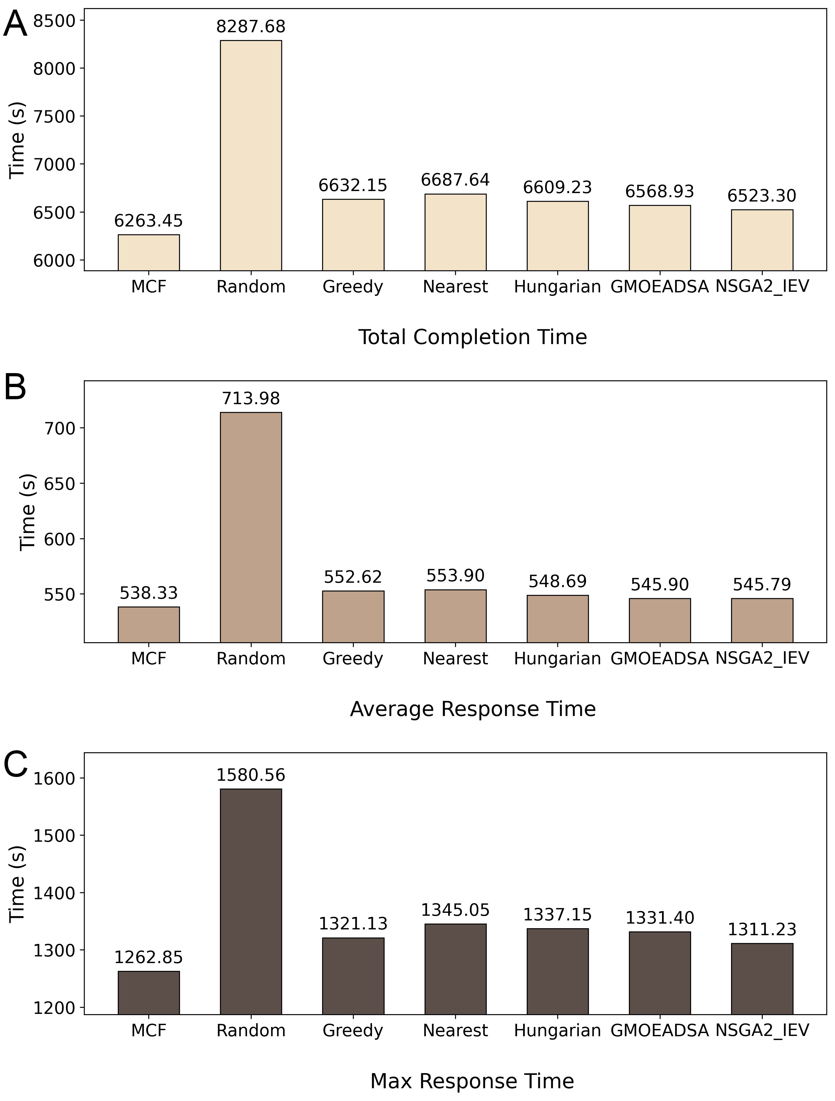
Figure 5. Performance comparison of different methods in terms of time-related metrics: (A) total completion time; (B) average response time; and (C) maximum response time. MCF: Minimum cost flow; G-MOEA/D-SA: Multiobjective Evolutionary Algorithm Based on Decomposition Using Simulated Annealing; NSGA-II-IEV: Non-dominated Sorting Genetic Algorithm II for the Integrated Emergency Vehicle Scheduling Model.
Figure 6 also confirms the adaptability of MCF across different task levels. MCF maintains lower response times at most levels, indicating that global joint scheduling can allocate limited emergency resources according to task demands. Its advantage is more evident for Level 1 tasks, where looser constraints provide a larger scheduling space and reduce unnecessary resource occupation. As the task level increases, high-quality vehicles and low-conflict routes become scarce, causing response times to rise and performance gaps to narrow. This indicates that high-level tasks impose greater scheduling pressure, making local rules or independent matching optimization less effective.
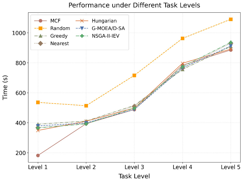
Figure 6. Comparison of different methods across task levels. MCF: Minimum cost flow; G-MOEA/D-SA: Multiobjective Evolutionary Algorithm Based on Decomposition Using Simulated Annealing; NSGA-II-IEV: Non-dominated Sorting Genetic Algorithm II for the Integrated Emergency Vehicle Scheduling Model.
To explain this increase in response time, Figure 7 shows the response-time distributions for Level 4 and Level 5 tasks, with each group based on 200 simulation runs. The boxes indicate the interquartile range (IQR, 25th–75th percentiles), the center lines indicate the median, the whiskers extend to the most extreme data points within 1.5 times the interquartile range below the first quartile and above the third quartile, and the circles denote outliers beyond the whiskers. The distributions shift upward and become wider, with higher upper bounds and more high-value outliers, indicating that resource competition amplifies extreme response delays. As high-quality resources are gradually occupied, later assignments are more likely to rely on suboptimal combinations, which increases response time. Consistent with the previous results, Random shows the highest distribution and largest fluctuations, revealing the risk of uncoordinated assignment under high-load scenarios. Although the other optimization methods improve average performance, their distributions become closer under resource scarcity. In contrast, MCF maintains a lower distribution, showing that it reduces the system-level impact of accumulated suboptimal assignments. Overall, Figure 5 to Figure 7 show that the proposed method improves response efficiency and scheduling stability under high-level tasks and high-load conditions.
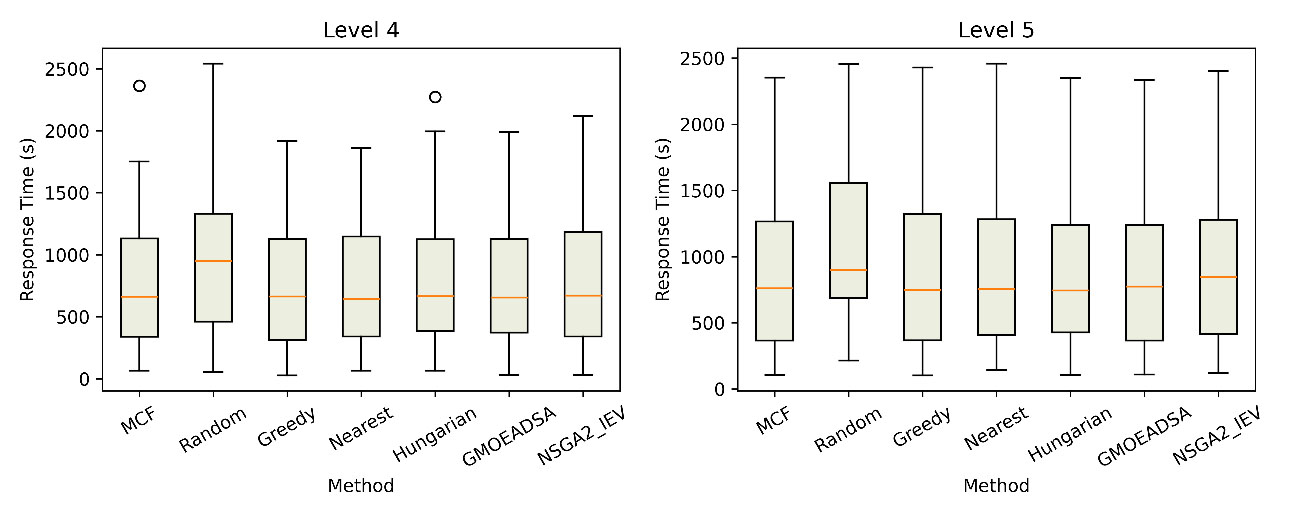
Figure 7. Response time distributions under high-level tasks (Levels 4–5). Each group contains n = 200 samples. The boxes represent the interquartile range (IQR, 25th–75th percentiles), the central lines indicate the median, the whiskers extend to the most extreme data points within 1.5 times the IQR from the lower and upper quartiles, and the circles represent outliers beyond the whiskers. MCF: Minimum Cost Flow; G-MOEA/D-SA: Multiobjective Evolutionary Algorithm Based on Decomposition Using Simulated Annealing; NSGA-II-IEV: Non-dominated Sorting Genetic Algorithm II for the Integrated Emergency Vehicle Scheduling Model.
Ablation study
Ablation settings
To evaluate the contribution of each component, an ablation study is conducted with four configurations. For the ablation study, all reported results are averaged over 1,000 independent experimental runs to reduce the influence of randomness in incident generation, traffic evolution, and scheduling decisions.
• I: The full model integrates DAGWN-based route generation with the proposed scheduling method.
• II: DAGWN-based candidate route generation is used with NSGA-II-IEV-based task assignment.
• III: The proposed scheduling method with the designed cost function is applied to static shortest routes.
• IV: The baseline combines static shortest route planning with NSGA-II-IEV-based task assignment.
Results and discussion
The full model achieves the best results in both Figures 8 and 9, demonstrating the complementary effects of disturbance-aware route generation and collaborative scheduling. Method II reduces average response time after introducing DAGWN-based candidate routes, indicating that incident disturbance information improves route quality and supports more effective route selection under affected traffic conditions. Method III improves total completion time and maximum response time by applying the proposed scheduling strategy to static shortest routes, showing that collaborative scheduling optimizes vehicle-task-route assignment and reduces extreme response delays. When used separately, route generation lacks global resource coordination, while scheduling optimization is constrained by static route quality; thus, neither component can achieve the best performance across all metrics. In contrast, the full model combines DAGWN-based disturbance-aware routes with MCF-based task assignment under limited resources, improving both route quality and scheduling performance. These results validate the effectiveness of the proposed hierarchical collaborative optimization framework for system-level CER response optimization.
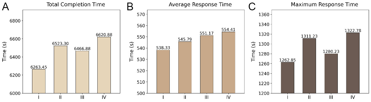
Figure 8. Time comparison of different ablation settings. (A) comparison of the total completion time under configurations I–IV, reflecting the overall efficiency of completing all emergency tasks; (B) comparison of the average response time, indicating the mean response efficiency across tasks; and (C) comparison of the maximum response time, representing the worst-case response delay.
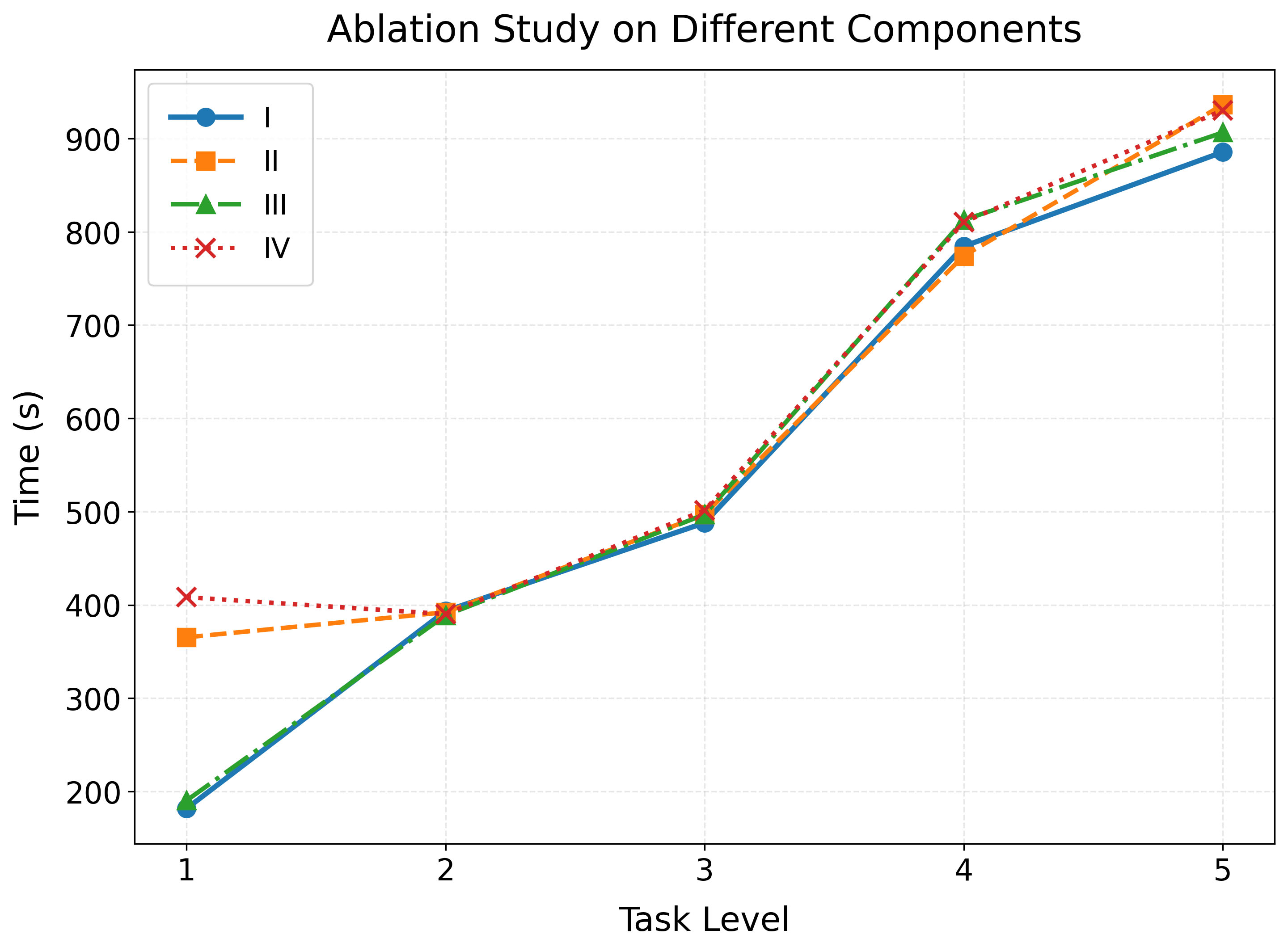
Figure 9. Performance comparison under different ablation settings across task levels.
These ablation results also support the modular design of the proposed framework. The proposed scheduling method can still operate with static shortest routes, indicating that the upper-layer optimizer is independent of a specific lower-layer predictor. Meanwhile, replacing static routes with DAGWN-based disturbance-aware candidate routes further improves scheduling performance, showing that the lower layer provides beneficial route-level information rather than introducing uncontrolled coupling. Therefore, the hierarchical design enables both independent operability of each layer and complementary performance gains when the two layers are integrated.
CONCLUSIONS
This paper investigates EV routing and scheduling in CER scenarios, where dynamic traffic disturbances and multi-task competition affect emergency response efficiency. We propose a disturbance-aware hierarchical framework that integrates traffic prediction, candidate route generation, and cost-based collaborative scheduling into a unified decision process. By modeling incident-induced disturbance propagation, the proposed method transforms prediction results into route and scheduling decisions, enabling coordinated optimization under dynamic traffic conditions. Future work will incorporate real traffic and incident data, evaluate more diverse road networks and incident scenarios, and explore real-time deployment in large-scale emergency response systems.
DECLARATIONS
Authors’ contributions
Made substantial contributions to the conception and design of the study: Gao, J.; Wu, C.
Developed the methodology, constructed the model, and designed the experimental framework: Gao, J.; Chen, Y.; Wu, C.
Performed data acquisition, simulation implementation, and experimental validation: Gao, J.; Zhong, L.; Lin, Y.
Performed data analysis and interpretation: Gao, J.; Chen, Y.
Drafted the manuscript: Gao, J.; Wu, C.
Provided administrative, technical, and material support: Wu, C.; Zhong, L.; Lin, Y.; Djahel, S.
Critically revised the manuscript for important intellectual content: Djahel, S.
All authors reviewed and approved the final manuscript.
Availability of data and materials
The road network data used in this study were obtained from publicly available OpenStreetMap data. The dataset for the study area can be accessed through the following Overpass API link: https://overpass-api.de/api/map?bbox=139.68421,35.67933,139.73373,35.71725. The processed datasets and simulation data generated during the current study are available from the corresponding author upon reasonable request.
AI and AI-assisted tools statement
During the preparation of this manuscript, the AI tool ChatGPT (version GPT-5.5 Thinking, released 2026-04-23) was used solely for language editing. The tool did not influence the study design, data collection, analysis, interpretation, or the scientific content of the work. All authors take full responsibility for the accuracy, integrity, and final content of the manuscript.
Financial support and sponsorship
None.
Conflicts of interest
Wu, C. is the Deputy Editor-in-Chief of Intelligent Networking and Computing. Zhong, L. is affiliated with Toyota Motor Corporation. Neither of them was involved in any part of the editorial process for this manuscript, including reviewer selection, manuscript handling, or editorial decision-making. The other authors declare that they have no conflicts of interest.
Ethical approval and consent to participate
Not applicable.
Consent for publication
Not applicable.
Copyright
© The Author(s) 2026.
REFERENCES
1. Fire and Disaster Management Agency, Ministry of Internal Affairs and Communications, Japan. Publication of the 2025 Edition of Current Status of Emergency and Rescue Services. Available online: https://www.soumu.go.jp/main_content/001050772.pdf. [accessed 26 July 2026].
2. Do-Duy, T.; Nguyen, L. D.; Duong, T. Q.; Khosravirad, S. R.; Claussen, H. Joint optimisation of real-time deployment and resource allocation for UAV-aided disaster emergency communications. IEEE. J. Select. Areas. Commun. 2021, 39, 3411-24.
3. Lu, L.; Wang, S. Literature review of analytical models on emergency vehicle service: location, dispatching, routing and preemption control. In 2019 IEEE Intelligent Transportation Systems Conference - ITSC, Auckland, New Zealand, October 27-30, 2019; IEEE, 2019, pp 3031-6. DOI: 10.1109/ITSC.2019.8916885.
4. Wu, J.; Kulcsár, B.; Ahn, S.; Qu, X. Emergency vehicle lane pre-clearing: From microscopic cooperation to routing decision making. Transp. Res. Part. B. Methodol. 2020, 141, 223-39.
5. Peelam, M. S. Naren; Gera, M.; Chamola, V.; Zeadally, S. A review on emergency vehicle management for intelligent transportation systems. IEEE. Trans. Intell. Transport. Syst. 2024, 25, 15229-46.
6. Heda, M.; Sophie Busch, J.; Aziz Sepa Seid Mayo, A.; Ermakova, T. RescueRoute: using real-time traffic data for routing emergency vehicles. In 2023 IEEE International Conference on Web Intelligence and Intelligent Agent Technology (WI-IAT), Venice, Italy, October 26-29, 2023; IEEE, 2023, pp 362-6.
7. Vikruthi, S.; Singasani, T. R.; M, V. T. R. P. K.; Nagendrudu, P. V. V. S. D.; Raghavendra, C.; Sahith, R. Detection of emergency vehicles in traffic and assign traffic free path using deep learning. In 2025 4th International Conference on Sentiment Analysis and Deep Learning (ICSADL), Bhimdatta, Nepal, February 18-20, 2025; IEEE, 2025, pp 1252-61.
8. Kim, J.; Sohn, K. Emergency response vehicle routing allowing lane straddling in congested traffic conditions under connected and autonomous vehicle environment. Transp. Res. Part. B. Methodol. 2025, 40, 6552-76.
9. Zlatkovic, M.; Cvijovic, Z.; Stevanovic, A.; Song, Y. Concepts of signal control preemption for emergency vehicles in connected vehicle environments. J. Road. Traffic. Eng. 2023, 69, 1-7.
10. Roy, S.; Hunter, M.; Saroj, A.; Guin, A. Development of emergency vehicle preemption strategies on smart corridors in a digital twin environment. In SIGSPATIAL '24: The 32nd ACM International Conference on Advances in Geographic Information Systems, Atlanta GA USA; ACM: New York, NY, USA, 2025, pp 12-21.
11. Moumen, I.; Zogarh, M.; Oukassou, Y.; Kobbane, A.; Rafalia, N.; Abouchabaka, J. CNN-GA approach for priority recognition and traffic signal optimization in urban emergency response. Procedia. Comput. Sci. 2025, 270, 4786-95.
12. Shaaban, K.; Khan, M. A.; Hamila, R.; Ghanim, M. A strategy for emergency vehicle preemption and route selection. Arab. J. Sci. Eng. 2019, 44, 8905-13.
13. Lin, P.; Chen, Z.; Pei, M.; Ding, Y.; Qu, X.; Zhong, L. Multiple emergency vehicle priority in a connected vehicle environment: a cooperative method. IEEE. Trans. Intell. Transport. Syst. 2024, 25, 173-88.
14. Li, Y.; Yu, R.; Shahabi, C.; Liu, Y. Diffusion convolutional recurrent neural network: data-driven traffic forecasting. In International Conference on Learning Representations (ICLR), Vancouver, Canada, April 30-May 3, 2018. Available online: https://openreview.net/forum?id=SJiHXGWAZ.
15. Yu, B.; Yin, H.; Zhu, Z. Spatio-temporal graph convolutional networks: a deep learning framework for traffic forecasting. In Twenty-Seventh International Joint Conference on Artificial Intelligence {IJCAI-18}, Stockholm, Sweden, July 13-19, 2018; International Joint Conferences on Artificial Intelligence Organization: California, 2018, pp 3634-40.
16. Wu, Z.; Pan, S.; Long, G.; Jiang, J.; Zhang, C. Graph WaveNet for Deep Spatial-Temporal Graph Modeling. In Twenty-Eighth International Joint Conference on Artificial Intelligence {IJCAI-19}, Macao, China, August 10-16, 2019; International Joint Conferences on Artificial Intelligence Organization: California, 2019, pp 1907-13.
17. Li, F.; Feng, J.; Yan, H.; et al. Dynamic Graph Convolutional Recurrent Network for traffic prediction: benchmark and solution. ACM. Trans. Knowl. Discov. Data. 2023, 17, 1-21.
18. Liu, H.; Dong, Z.; Jiang, R.; et al. Spatio-Temporal Adaptive Embedding Makes Vanilla Transformer SOTA for Traffic Forecasting. In CIKM '23: The 32nd ACM International Conference on Information and Knowledge Management, Birmingham United Kingdom; ACM: New York, NY, USA, 2023, pp 4125-9.
19. Qiu, Z.; Zhu, T.; Jin, Y.; Sun, L.; Du, B. A graph attention fusion network for event-driven traffic speed prediction. Inf. Sci. 2023, 622, 405-23.
20. Zheng, Y.; Luo, J.; Hu, M. Spatial-temporal incident-aware dynamic graph convolution networks for traffic flow prediction. Expert. Syst. Appl. 2026, 305, 130689.
21. Hemici, M.; Zouache, D.; Brahmi, B.; Got, A.; Drias, H. A decomposition-based multiobjective evolutionary algorithm using Simulated Annealing for the ambulance dispatching and relocation problem during COVID-19. Appl. Soft. Comput. 2023, 141, 110282.
22. Zhen, L.; Wu, J.; Chen, F.; Wang, S. Traffic emergency vehicle deployment and dispatch under uncertainty. Transp. Res. Part. E. Logist. Transp. Rev. 2024, 183, 103449.
23. Tan, Z.; Zhen, L.; Yang, Z.; Liu, L.; Fan, T. Multi-period emergency vehicle fleet redistribution and dispatching. Transportmetrica. A. Transp. Sci. 2025, 21, 2243344.
24. Nawaz, F.; Ornik, M. Multiagent, Multitarget path planning in Markov decision processes. IEEE. Trans. Automat. Contr. 2023, 68, 7560-74.
25. Li, X.; Wang, X.; Xu, J.; Chen, W.; Lyu, B. Integrated emergency vehicle scheduling model in urban emergency rescue within a time-limited period. Transp. Res. Rec. 2024, 2678, 802-18.
26. Cao, M.; Peng, J.; Yang, L.; Yang, Y. Multi-UAV task allocation and path planning in emergency rescue scenarios with uncertain requirements. J. Ind. Manag. Optim. 2025, 21, 6107-33.
27. Luzon, Y.; Baron, O.; Verter, V.; Berman, O. On designing a fire emergency vehicle fleet. M&SOM. 2025, 27, 1995-2015.
28. Gottschalg, G.; Haferkamp, J.; Ulmer, M. W.; Strauss, A. Dynamic matching for teleoperated car-sharing services. Transp. Sci. 2026, 60, 466-83.
Cite This Article
 Open Access
How to Cite
Download Citation
Export Citation File:
Type of Import
Tips on Downloading Citation
Citation Manager File Format
Type of Import
Direct Import: When the Direct Import option is selected (the default state), a dialogue box will give you the option to Save or Open the downloaded citation data. Choosing Open will either launch your citation manager or give you a choice of applications with which to use the metadata. The Save option saves the file locally for later use.
Indirect Import: When the Indirect Import option is selected, the metadata is displayed and may be copied and pasted as needed.
About This Article
Copyright

Data & Comments
Data
0





Comments
Comments must be written in English. Spam, offensive content, impersonation, and private information will not be permitted. If any comment is reported and identified as inappropriate content by OAE staff, the comment will be removed without notice. If you have any queries or need any help, please contact us at [email protected].