

Optimal maintenance policy for systems subject to random shocks: a semi-Markov decision process approach
 0
0 Graphical Abstract
Abstract
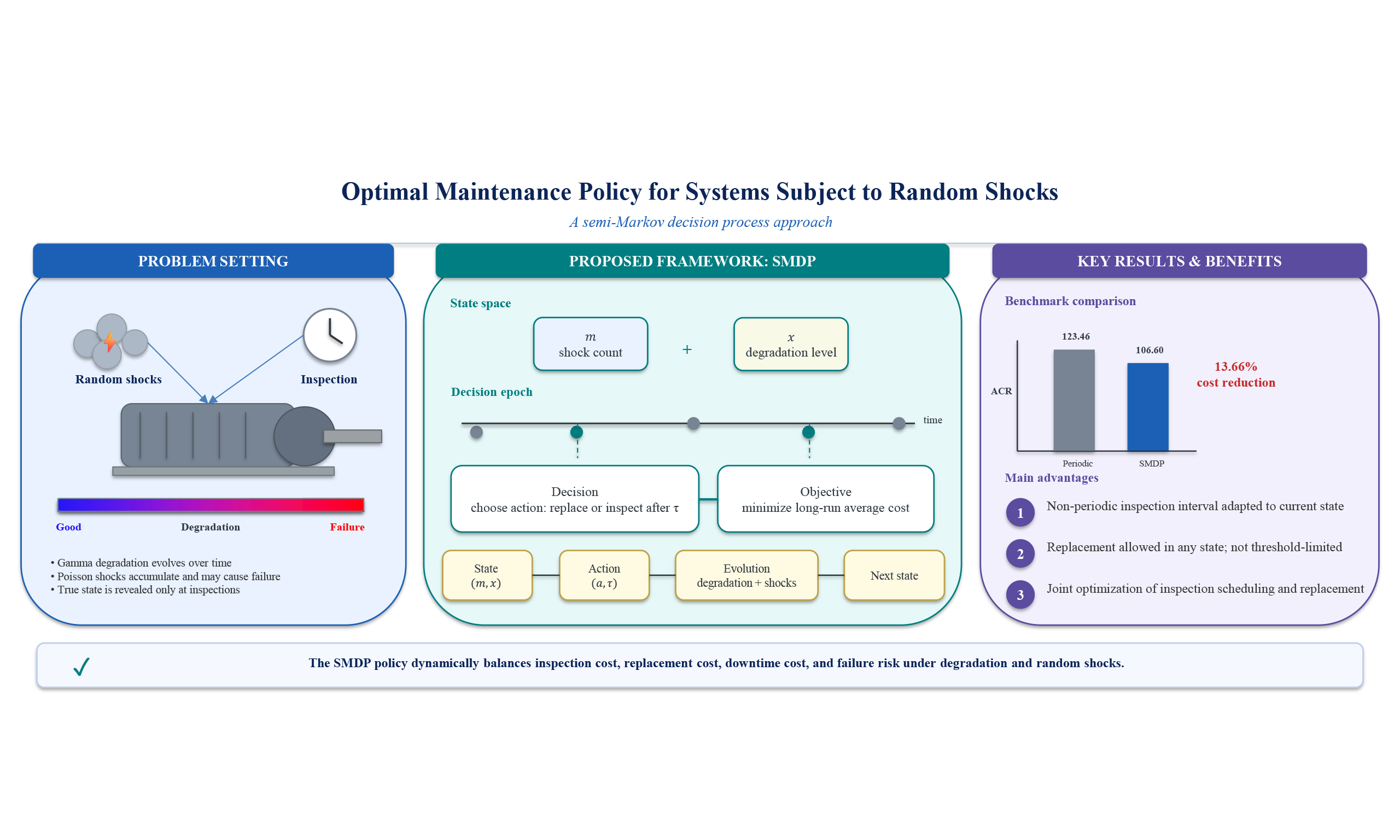
This paper studies an average-cost maintenance optimization problem for a single-component system subject to continuous degradation and random shocks. The degradation process is modeled by a Gamma process, while random shocks arrive according to a Poisson process. A system failure occurs when either the degradation level reaches or exceeds its failure threshold, or the accumulated number of shocks reaches the shock failure threshold. Since failures are non-self-announcing, both the failure state and the system condition can only be revealed through inspections. To reduce the long-run operating cost, we propose a state-dependent non-periodic inspection and replacement policy, where the next inspection interval and the replacement action are jointly optimized according to the current degradation level and accumulated shock state. A numerical algorithm based on state-space discretization and bisection search is developed to compute the optimal policy. Numerical results show that the proposed policy consistently outperforms the optimized periodic inspection and replacement benchmark, with average-cost-rate reductions ranging from 8.60% to 29.33% across the tested parameter settings. Sensitivity analysis further demonstrates that the proposed policy consistently outperforms the benchmark policy under different cost, shock, and degradation parameter settings. The results confirm that dynamically adjusting inspection intervals according to the system state can effectively balance inspection cost, downtime cost, and replacement cost.
Keywords


 Download PDF
1. INTRODUCTION
In practical industrial environments, engineering systems are often affected by multiple failure mechanisms. Internal degradation, such as wear, corrosion, fatigue, aging, and performance deterioration, typically progresses gradually over operating time. Meanwhile, external shocks caused by random loads, environmental disturbances, impacts, or abnormal operating conditions may occur unexpectedly during system operation. Such shocks may be harmless, accelerate the degradation process, cause recoverable damage, or directly lead to system failure. Therefore, it is necessary to inspect the system condition and implement appropriate maintenance or replacement actions to reduce failure risk, improve system availability, and control the long-run operating cost. This issue is particularly important for complex industrial systems whose failures may result in high downtime losses, safety risks, and maintenance expenses.
Periodic inspection policies have been widely studied in maintenance decision-making for engineering systems. For systems with a fixed inspection schedule, Cavalcante et al.[1] investigated an inspection and replacement policy in which maintenance opportunities occur at predetermined periodic visits, and analyzed how preventive replacement timing and visit frequency affect the cost rate, reliability, and availability. For redundant and standby systems, Wang et al.[2] studied redundancy optimization for cold-standby systems with degrading components under periodic inspection and preventive maintenance, while Golmohammadi and Ardakan[3] optimized reliability for systems with active and standby degrading components under a periodic inspection and maintenance policy. In addition, Levitin et al.[4] optimized a state-based software rejuvenation policy for real-time tasks under periodic inspections and time limitations. More recently, Ning et al.[5] jointly optimized preventive maintenance and the triggering mechanism of protective devices for k-out-of-n:F systems based on periodic inspection. Similar periodic inspection activities were also applied to homogeneous systems by Sharifi et al.[6,7,8], Bjarnason et al.[9,10,11], and Golmakani et al.[12,13]. These studies demonstrate the applicability of periodic inspection policies in different engineering systems. However, in practical applications, due to the dynamic changes in system states and the number of available components, fixed-period inspection may result in excessive maintenance or delayed inspection, thereby increasing maintenance costs or failure risks. To improve the flexibility of inspection decisions, recent studies have considered adaptive or non-periodic inspection policies. For example, Liu et al.[14] proposed a non-periodic inspection policy for k-out-of-n:G systems, where the next inspection interval is determined according to the observed system state. Esposito et al.[15] developed an adaptive maintenance policy in which imperfect and perfect inspections are used to determine replacement decisions and future replacement times. Wei et al.[16] formulated a belief-based SMDP for predictive inspection and maintenance of multi-state systems with non-periodic decision epochs. Najafi and Taghipour[17] jointly optimized inspection scheduling and imperfect maintenance within an SMDP framework by exploring a broader inspection-maintenance policy space. These studies show that non-periodic inspection can make better use of system-state information than traditional periodic inspection.
For systems mainly subject to internal degradation, inspection and maintenance optimization has been extensively studied. For example, Davies et al.[18] optimized inspection and maintenance planning for ship coating failures by modeling corrosion defects using a non-homogeneous Poisson process. Zhang et al.[19] studied a two-component degradation system with failure dependence and imperfect inspection under a dual periodic inspection policy. Zheng et al.[20] formulated a joint condition-based maintenance and spare provisioning problem for a K-out-of-N system as a Markov decision process. Liu et al.[21] proposed a condition-based maintenance policy for leased equipment with hybrid preventive maintenance and periodic inspection. Wang et al.[22] developed an inspection-based preventive maintenance strategy for k-out-of-n: G load-sharing systems with three-state components. These studies have enriched degradation-based maintenance modeling by considering stochastic degradation, imperfect inspection, spare provisioning, multi-state components, and system dependence. When external shocks are incorporated, the inspection and maintenance problem becomes more complicated because the system state may be affected by both continuous degradation and sudden shock-induced damage. Zhang et al.[23] analyzed a two-component system subject to natural degradation and zoned shocks, and proposed reliability-centered and shock-based maintenance strategies. Gan et al.[24] investigated systems with degradation-mitigation and shock-resistance subsystems, showing that subsystem interactions significantly influence reliability and maintenance optimization. Fischetti et al.[25] developed a two-level inspection and replacement policy for a three-stage failure process subject to natural degradation and external shocks. Zhang et al.[26] proposed a predictive maintenance scheduling method for recoverable stochastic hybrid systems under degradation and shock-induced common-cause failures. Li et al.[27] designed a group inspection and maintenance policy for heterogeneous multi-component systems subject to gradual degradation and random shocks. These recent studies demonstrate that degradation-shock interactions have received increasing attention in reliability and maintenance optimization. Other studies have investigated degradation- shock-dependent systems from different perspectives, including remaining useful life prediction[28], reliability analysis in dynamic environments[29], mission reliability modeling[30], and predictive maintenance scheduling[26]. However, existing models still rely on periodic or partially periodic inspection epochs, and their replacement policies are commonly based on fixed thresholds or predefined maintenance rules.
The above limitations may become more significant when the system experiences repeated shocks or reaches a high degradation level. In such cases, a fixed inspection interval may fail to respond to rapidly changing system conditions in time, while a threshold-based replacement rule may not fully capture the joint influence of degradation level, shock history, and future risk. Consequently, the resulting maintenance policy may be locally effective under a restricted decision structure but not globally optimal over the complete inspection and replacement policy space. This motivates the need for a more flexible decision framework in which both inspection timing and replacement actions can be optimized according to the current system state. To address this issue, this paper proposes a semi-Markov decision process (SMDP) framework for inspection and replacement optimization. Compared with conventional periodic inspection and threshold-based replacement policies, the main advantages of the proposed method are threefold:
1. The proposed method allows non-periodic inspection decisions to be made under arbitrary system states. The next inspection time is treated as an optimizable decision variable so that the inspection interval can be dynamically adjusted according to the current system condition.
2. Replacement actions can be directly selected in each system state. This differs from threshold-based replacement policies, where replacement is usually triggered only when a predefined degradation, reliability, or state threshold is reached.
3. Inspection scheduling and replacement decisions are jointly optimized within a unified SMDP framework. This allows for a comprehensive exploration of the entire policy space, leading to a globally optimal maintenance strategy that minimizes the long-run average cost.
2. MODEL DESCRIPTION
In this section, we present the model assumptions and formulate the basic quantities, including the system transition probabilities and the mean downtime duration, which provide the foundation for the subsequent maintenance optimization model.
2.1 Notation
The notation used throughout the model is summarized in Table 1.
Notation used in the model
| Notation | Description |
| Poisson arrival process of random shocks up to time t | |
| λ | Arrival rate of random shocks |
| m | Accumulated number of shocks |
| M | Failure threshold for the accumulated number of shocks |
| x | Degradation level of the system |
| L | Degradation failure threshold |
| Transition probability from shock state m to shock state | |
| Degradation-induced failure probability within an interval of length t, starting from degradation level x | |
| Failure probability within an interval of length t, starting from state | |
| Mean downtime duration within an inspection interval of length t | |
| Non-periodic inspection action with inspection interval t | |
| Immediate replacement action | |
| π | Maintenance policy |
| Inspection cost | |
| Downtime cost rate | |
| Preventive replacement cost | |
| Corrective replacement cost | |
| Expected cost from state | |
| Expected elapsed time from state | |
| g ( | Candidate (optimal) average cost rate |
| Optimal excess-cost function under candidate cost rate g | |
| Optimal non-periodic inspection interval at state |
2.2 Assumptions
The system under consideration is a single-component system that undergoes continuous degradation and random shocks. The key assumptions of the model are as follows:
1. Random shocks occur according to a Poisson process
2. The degradation increment over an interval of length t follows a Gamma distribution with shape parameter
3. The degradation process and the shock process are independent of each other;
4. A system fails when the accumulated number of shocks reaches the failure threshold M or the degradation level reaches or exceeds the threshold L, whichever occurs first;
5. Failures are non-self-announcing; the failure status, accumulated shock count, and degradation level can only be revealed through inspections.
Remark 1. The independence assumption is adopted to establish a tractable baseline model for the joint optimization of inspection scheduling and replacement decisions. It is suitable for engineering systems in which internal degradation is mainly caused by gradual physical deterioration, such as wear, corrosion, fatigue, or aging, while external shocks are caused by random environmental or operational disturbances. Under this assumption, the degradation-induced failure event and the shock-induced failure event can be modeled as two competing failure mechanisms with explicit transition probabilities. Nevertheless, this assumption may not hold for systems with strong degradation-shock dependence. For example, shocks may accelerate the degradation process, and a high degradation level may increase the system's vulnerability to shocks. Such dependence is beyond the scope of the present study and is left for future research.
Remark 2. The present model assumes that inspections are perfect, meaning that the accumulated shock state and the degradation level can be accurately observed at each inspection epoch. This assumption is commonly used as a baseline setting for inspection-based maintenance optimization because it allows the state-dependent inspection interval and replacement decision to be explicitly characterized. In practice, however, inspections may be subject to measurement errors, missed detections, or delayed fault identification. Incorporating such inspection uncertainty would require the observed state to be replaced by a belief state or an estimated degradation distribution, leading to a partially observable decision model. This extension is meaningful but beyond the scope of the present study.
Define the system state as a two-dimensional vector
Accordingly, the degradation-induced failure probability within an interval of length t, starting from degradation level x, can be expressed by the upper tail probability of the Gamma distribution[31]:
2.3 Transition probability
For a Poisson shock process, the inter-arrival times are independent and identically distributed exponential random variables, and the arrival time of the l-th shock follows an Erlang distribution[32]. Therefore, for
The corresponding cumulative distribution function is[32]
Next, let
1. If
2. If
3. If
2.4 Mean downtime duration
Let
Let
3. AVERAGE-COST OPTIMAL MAINTENANCE POLICY
3.1 Maintenance actions and renewal equations
In this section, we formulate the average-cost optimal maintenance problem. Two types of maintenance actions are considered: non-periodic inspection, denoted by
Both actions are admissible at any non-failed system state
1. If action
2. If action
Under a given maintenance policy π, let
The recursive expressions for
1. If policy π prescribes action
2. If policy π prescribes action
where
3.2 Excess-cost Bellman optimality equation
To derive the optimal maintenance policy, we follow the standard average-cost Markov decision process framework and transform the average-cost problem into a parametric excess-cost problem[33]. Let g denote a candidate average cost rate. For each non-failed state
If immediate replacement
If non-periodic inspection
For a fixed candidate cost rate g, the optimal inspection interval associated with the non-periodic inspection action is obtained by
and the minimized g-adjusted cost of non-periodic inspection is
For a fixed candidate average cost rate g, the original average-cost problem is converted into an excess-cost minimization problem. At each decision epoch, the decision maker needs to compare only the g-adjusted costs of the two admissible action types: immediate replacement and non-periodic inspection. The former terminates the current renewal cycle immediately, whereas the latter incurs the inspection cost, the expected downtime cost, the time-adjusted term
This equation is valid because the next decision depends on the past history only through the observed state
Otherwise, non-periodic inspection is optimal, and the corresponding inspection interval is
After discretization, the transition structure permits a backward recursion because both the accumulated shock count and the degradation level are nondecreasing. After setting the boundary values for the failed states, the non-failed grid states are evaluated from larger to smaller values of m and x. The optimal maintenance policy is then obtained by comparing the two action values at each state.
3.3 Determination of the optimal average cost rate
The value of g in Eq. (14) is only a candidate average cost rate. Therefore, solving Eq. (14) for a given g yields the policy that is optimal with respect to this candidate benchmark, but it does not directly determine the optimal average cost rate. To identify the true optimal average cost rate, we examine the optimal excess cost at the renewal state (0, 0).
For any admissible maintenance policy π, the expected excess cost of one renewal cycle under the candidate cost rate g is
Equivalently,
Since
After optimizing over all admissible policies, the optimal excess cost at the renewal state equals
Thus,
Consequently, the optimal average cost rate
At this root,
The optimal maintenance policy is then obtained from Eq. (14) by setting
3.4 Numerical implementation and convergence check
The continuous degradation state is discretized on a uniform grid over
For a fixed candidate average cost rate g, the discretized Bellman equation is solved recursively over the state space. Boundary values are first assigned to failed states with
4. NUMERICAL EXAMPLE
In this section, the performance of the proposed maintenance policy is validated by a numerical example. We consider an engineering system operating in a random environment, subject to both internal degradation and external shocks during its service life. The internal degradation process represents gradual deterioration caused by aging, wear, corrosion, or fatigue, while external shocks represent sudden environmental or operational disturbances that independently contribute to shock-induced failure in the present model. The system state cannot be continuously observed and can be revealed only through inspections. Parameters used in the numerical example are shown in Table 2. Here, M denotes the failure threshold for the accumulated number of shocks, λ is the arrival rate of external shocks, α is the shape-rate coefficient of the Gamma process, and β is the Gamma rate parameter. The degradation failure threshold is denoted by L. In addition,
Parameters used in the policy
| λ | α | β | ||||||
| 5 | 0.1 | 1.1 | 2.7 | 12 | 4000 | 1000 | 2000 | 100 |
4.1 Results for the proposed policy
Based on the baseline parameter setting, the optimal average cost rate is obtained by solving the root equation
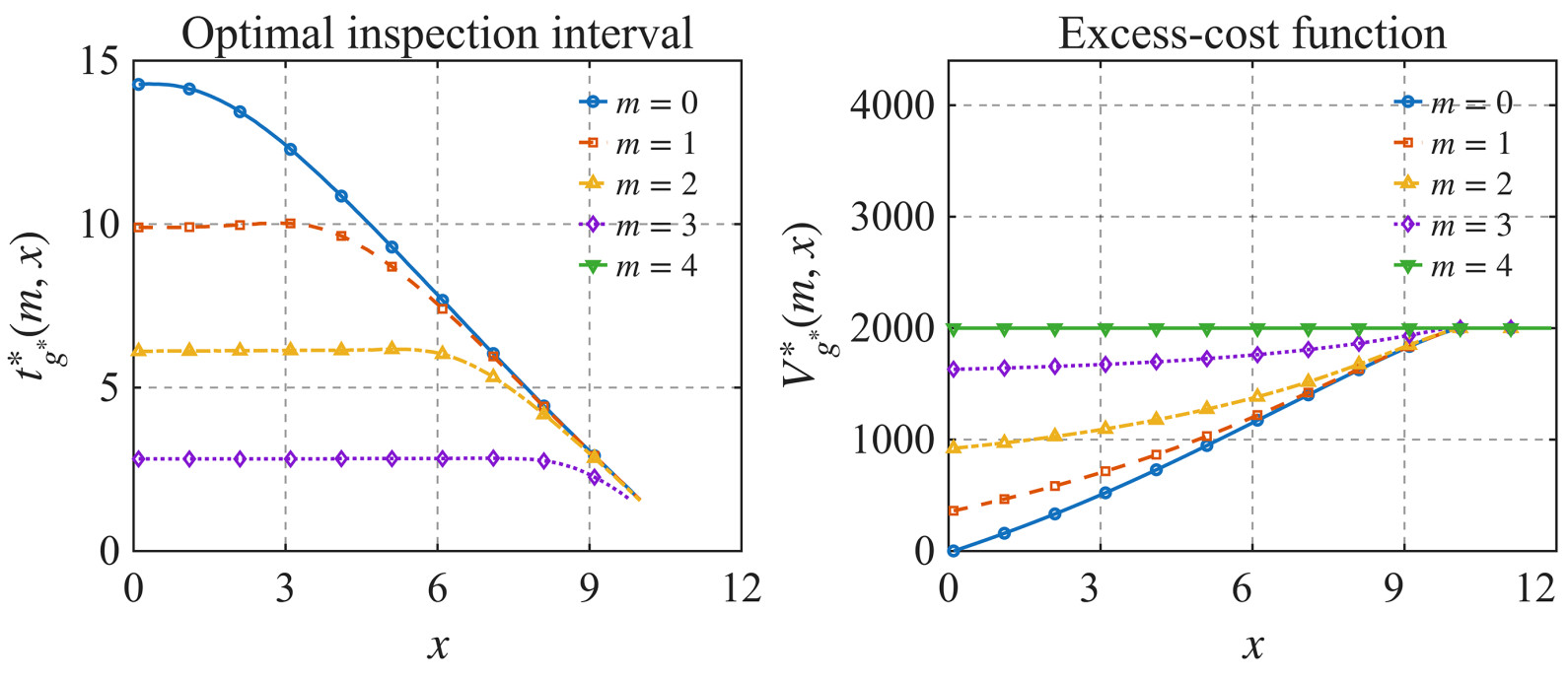
Figure 1. Optimal inspection intervals (left panel) and excess-cost function (right panel) for different operating states. The shock-failure state m=M=5 is excluded because the inspection interval is not optimized after failure.
The left panel of Figure 1 shows that the optimal inspection interval is strongly state-dependent. For a fixed accumulated shock state m, the inspection interval generally decreases as the degradation level x increases, because the system approaches the degradation failure threshold and requires more frequent inspections to reduce the expected downtime caused by non-self-announcing failures. Similarly, for a fixed degradation level, the inspection interval tends to decrease as m increases, because the system approaches the shock failure threshold. Thus, the policy becomes more conservative as the system deteriorates. When both m and x are small, the system is relatively healthy, allowing longer inspection intervals, which helps avoid unnecessary inspection costs. By contrast, when the system approaches either the shock failure threshold or the degradation failure threshold, the inspection interval becomes shorter, and immediate replacement is selected in states where no inspection interval is plotted. Therefore, the proposed policy adaptively balances inspection cost, downtime cost, and replacement cost according to the observed system state. In particular, because the baseline threshold is
Remark 4. To examine the influence of discretization error, the computation was repeated using different grid resolutions for both the degradation state and the inspection interval. The relative difference is computed with respect to the baseline grid, i.e.,
Sensitivity of the optimal average cost rate to discretization steps
| ACR | Relative difference from baseline | ||
| 0.20 | 0.02 | 108.56 | 1.84% |
| 0.10 | 0.01 | 106.60 | Baseline |
| 0.05 | 0.005 | 106.54 | 0.06% |
4.2 Comparison with a benchmark policy
To evaluate the effectiveness of the proposed state-dependent non-periodic inspection policy, we compare it with a benchmark periodic inspection and replacement policy[34,35], denoted by Policy B. Under Policy B, inspections are performed at a fixed interval T, and preventive replacement is conducted when the observed degradation level reaches or exceeds a predetermined threshold
Table 4 reports the optimal benchmark policy and its performance. The optimal periodic inspection interval is
Optimal periodic inspection and replacement policy
| 5.00 | 8.70 | 123.46 | 13.66% |
where
As shown in Table 4, the proposed policy reduces the average cost rate by 13.66% compared with the optimized benchmark policy. This improvement is mainly due to the state-dependent structure of the proposed policy. Unlike the benchmark policy, which uses a fixed inspection interval regardless of the current system condition, the proposed policy dynamically adjusts the next inspection interval according to both the accumulated number of shocks m and the degradation level x. When the system is close to either the shock failure threshold or the degradation failure threshold, the proposed policy shortens the inspection interval to reduce the risk of undetected failure and the associated downtime cost. Conversely, when the system is in a relatively healthy state, longer inspection intervals can be adopted to avoid unnecessary inspection costs. Therefore, the proposed policy achieves a better balance among inspection cost, downtime cost, and replacement cost.
4.3 Sensitivity analysis
To examine the robustness of the proposed policy and to understand the effects of different model parameters, a sensitivity analysis is conducted. Starting from the baseline parameter setting in Table 2, each parameter is varied individually while all the other parameters are kept unchanged. Specifically, each parameter is multiplied by 0.5, 0.75, 1.0, 1.25, and 1.5, respectively. For the shock threshold M, the adjusted value is rounded upward to the nearest integer.
Table 5 reports the average cost rate of the proposed policy under each parameter setting. The value in parentheses represents the percentage reduction in average cost rate compared with the optimized benchmark policy under the same parameter setting. Several observations can be obtained from Table 5. First, the proposed policy consistently outperforms the benchmark policy for all parameter settings, as all reported cost-rate reductions are positive. This confirms the robustness of the proposed state-dependent policy. Second, the optimal average cost rate increases with the cost parameters
Comparison of average cost rates under different parameter settings
| Parameter | -50% | -25% | Baseline | +25% | +50% |
| 98.54 (14.41%) | 103.26 (13.88%) | 106.60 (13.66%) | 109.29 (13.54%) | 111.58 (13.49%) | |
| 104.15 (11.79%) | 105.50 (12.67%) | 106.60 (13.66%) | 107.54 (14.66%) | 108.36 (15.66%) | |
| 65.11 (19.35%) | 86.75 (15.61%) | 106.60 (13.66%) | 125.59 (12.16%) | 143.70 (10.95%) | |
| 99.15 (12.61%) | 103.13 (12.94%) | 106.60 (13.66%) | 109.73 (14.58%) | 112.59 (15.63%) | |
| M | 159.33 (16.81%) | 123.27 (15.17%) | 106.60 (13.66%) | 95.28 (16.35%) | 94.13 (13.46%) |
| λ | 94.90 (13.29%) | 99.10 (13.11%) | 106.60 (13.66%) | 116.36 (15.43%) | 127.93 (17.59%) |
| α | 80.29 (29.33%) | 91.19 (20.05%) | 106.60 (13.66%) | 124.60 (11.39%) | 144.53 (10.92%) |
| β | 202.01 (8.60%) | 134.51 (10.51%) | 106.60 (13.66%) | 92.93 (18.63%) | 85.66 (23.73%) |
To further illustrate how the optimal policy changes with parameter variations, Figures 2 and 3 plot the optimal inspection interval
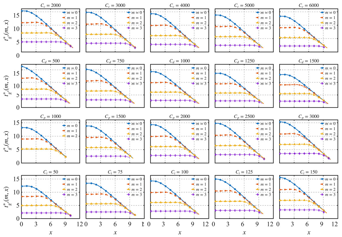
Figure 2. Sensitivity of the optimal inspection interval with respect to cost parameters. Different curves represent different accumulated shock states m and are distinguished by line styles and markers.
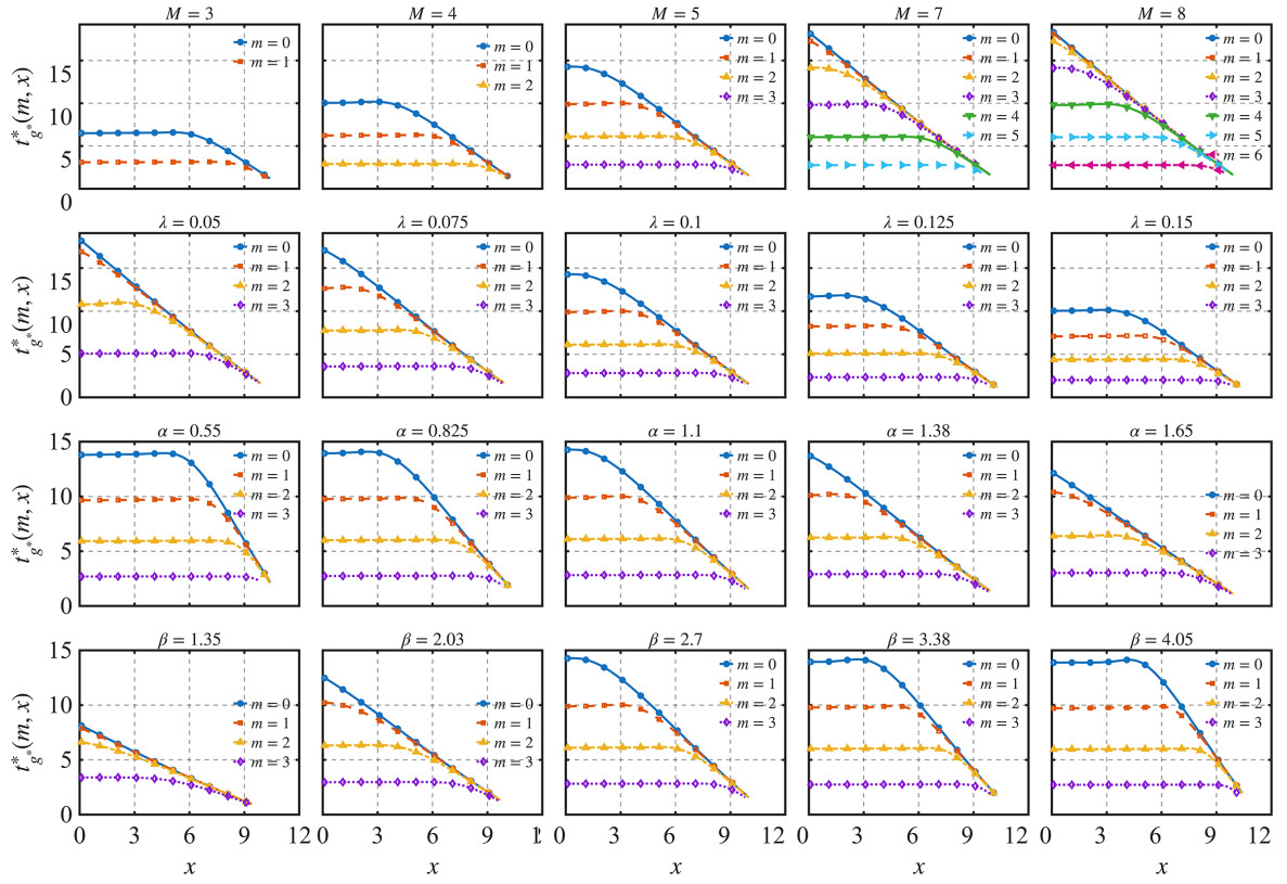
Figure 3. Sensitivity of the optimal inspection interval with respect to shock and degradation parameters. Different curves represent different accumulated shock states m and are distinguished by line styles and markers.
Figure 2 shows that the cost parameters affect the inspection policy in different ways. As
Figure 3 further confirms the influence of the shock and degradation parameters. When M increases, more shock states are allowed before failure, and the policy includes more curves corresponding to larger values of m. For smaller m, the system is relatively far from the shock failure boundary, and longer inspection intervals are permitted. As λ increases, shocks arrive more frequently, and the optimal inspection intervals become shorter. For the degradation parameters, a larger α leads to faster degradation and thus shorter inspection intervals. In contrast, a larger β slows down the degradation process under the rate-parameter formulation, so the optimal inspection intervals become longer.
Overall, the sensitivity analysis shows that the proposed policy can adaptively respond to changes in both economic and stochastic parameters. The policy schedules shorter inspection intervals when failure risk or failure-related costs increase, and longer inspection intervals when inspections or preventive replacements become more expensive or when the degradation process becomes less severe. These results demonstrate the flexibility of the proposed non-periodic inspection policy and explain its consistent advantage over the benchmark periodic policy.
5. CONCLUSION
This paper investigated an average-cost maintenance optimization problem for a single-component system subject to both continuous degradation and random shocks. The degradation process was modeled as a Gamma process, and the shock arrivals were described by a Poisson process. Since failures are non-self-announcing, the system condition can only be identified at inspection epochs. Under this setting, a state-dependent non-periodic inspection and replacement policy was proposed, in which both the inspection interval and the replacement action are optimized according to the current accumulated shock state and degradation level. The maintenance problem was formulated within a semi-Markov decision process framework. By introducing a candidate average cost rate, the original long-run average-cost problem was converted into an excess-cost Bellman optimality equation, and the optimal action at each state was obtained by comparing the adjusted cost of immediate replacement with that of non-periodic inspection. This formulation enables the joint optimization of inspection timing and replacement decisions over the entire state space.
Several extensions can be considered in future research. First, the present model assumes perfect inspections, where the accumulated shock state and degradation level can be accurately observed at inspection epochs. Future work may incorporate imperfect inspections, measurement errors, missed detections, or delayed fault identification. In that case, the decision process would need to be formulated using belief states or partially observable information. Second, the shock process and degradation process are assumed to be independent. In practical systems, random shocks may accelerate degradation, and degradation may also increase the system's vulnerability to shocks. Modeling such dependence would make the policy more realistic. Third, this study considers immediate replacement as the only maintenance action that restores the system condition. Future studies may introduce imperfect or partial maintenance actions, such as minor repair, degradation reduction, or shock-resistance improvement, by expanding the action space and modifying the corresponding transition probabilities and maintenance costs. Finally, parameter uncertainty and online learning can be incorporated to develop adaptive maintenance policies when the degradation and shock parameters are not fully known in advance.
DECLARATIONS
Authors' contributions
Made substantial contributions to the conception and design of the study, model formulation, numerical analysis, and manuscript writing: Liu, Y.
Contributed to model development, interpretation of results, manuscript revision, and supervision: Zhao, X.
Both authors read and approved the final manuscript.
Availability of data and materials
The original contributions and numerical results presented in this study are included in the article. Further inquiries can be directed to the corresponding author.
AI and AI-assisted tools statement
During the preparation of this manuscript, the AI tool ChatGPT (version 5.5, released June 2023) was used solely for language editing. The tool did not influence the study design, data collection, analysis, interpretation, or the scientific content of the work. All authors take full responsibility for the accuracy, integrity, and final content of the manuscript.
Financial support and sponsorship
None.
Conflicts of interest
Both authors declared that there are no conflicts of interest.
Ethical approval and consent to participate
Not applicable.
Consent for publication
Not applicable.
Copyright
© The Author(s) 2026.
REFERENCES
1. Cavalcante, C. A. V.; Lopes, R. S.; Scarf, P. A. Inspection and replacement policy with a fixed periodic schedule. Reliab. Eng. Syst. Saf. 2021, 208, 107402.
2. Wang, W.; Wu, Z.; Xiong, J.; Xu, Y. Redundancy optimization of cold-standby systems under periodic inspection and maintenance. Reliab. Eng. Syst. Saf. 2018, 180, 394-402.
3. Golmohammadi, E.; Ardakan, M. A. Reliability optimization problem with the mixed strategy, degrading components, and a periodic inspection and maintenance policy. Reliab. Eng. Syst. Saf. 2022, 223, 108500.
4. Levitin, G.; Xing, L.; Xiang, Y. Optimizing software rejuvenation policy for tasks with periodic inspections and time limitation. Reliab. Eng. Syst. Saf. 2020, 197, 106776.
5. Ning, R.; Wang, X.; Zhao, X.; Li, Z. Joint optimization of preventive maintenance and triggering mechanism for k-out-of-n: F systems with protective devices based on periodic inspection. Reliab. Eng. Syst. Saf. 2024, 251, 110396.
6. Sharifi, M.; Taghipour, S.; Abhari, A. Inspection interval optimization for a k-out-of-n load sharing system under a hybrid mixed redundancy strategy. Reliab. Eng. Syst. Saf. 2021, 213, 107681.
7. Sharifi, M.; Taghipour, S.; Abhari, A. Condition-based optimization of non-identical inspection intervals for a k-out-of-n load sharing system with hybrid mixed redundancy strategy. Knowl. Based. Syst. 2022, 240, 108153.
8. Sharifi, M.; Taghipour, S. Optimal inspection interval for a k-out-of-n system with non-identical components. J. Manuf. Syst. 2020, 55, 233-47.
9. Bjarnason, E. T. S.; Taghipour, S. Periodic inspection frequency and inventory policies for a k-out-of-n system. IIE. Trans. 2016, 48, 638-50.
10. Bjarnason, E. T. S.; Taghipour, S.; Banjevic, D. Joint optimal inspection and inventory for a k-out-of-n system. Reliab. Eng. Syst. Saf. 2014, 131, 203-15.
11. Bjarnason, E. T. S.; Taghipour, S. Optimizing simultaneously inspection interval and inventory levels
12. Golmakani, H. R.; Fattahipour, F. Optimal replacement policy and inspection interval for condition-based maintenance. Int. J. Prod. Res. 2011, 49, 5153-67.
13. Golmakani, H. R.; Moakedi, H. Periodic inspection optimization model for a two-component repairable system with failure interaction. Comput. Ind. Eng. 2012, 63, 540-5.
14. Liu, Y.; Wang, G.; Liu, P. A condition-based maintenance policy with non-periodic inspection for k-out-of-n: G systems. Reliab. Eng. Syst. Saf. 2024, 241, 109640.
15. Esposito, N.; Piscopo, A.; Castanier, B.; Giorgio, M. An adaptive maintenance policy for degrading units with an imperfect and a perfect inspection. Eur. J. Oper. Res. 2026, 330, 139-56.
16. Wei, Y.; Li, A.; Li, Y.; Cheng, Y. An optimal predictive inspection and maintenance policy for a multi-state system: a belief-based SMDP approach. Reliab. Eng. Syst. Saf. 2026, 265, 111497.
17. Najafi, S.; Taghipour, S. Joint optimization of inspection scheduling and imperfect maintenance under stochastic repair effects and regime-dependent feasibility. Comput. Ind. Eng. 2026, 218, 112109.
18. Davies, J.; Truong-Ba, H.; Cholette, M. E.; Will, G. Optimal inspections and maintenance planning for anti-corrosion coating failure on ships using non-homogeneous Poisson Processes. Ocean. Eng. 2021, 238, 109695.
19. Zhang, N.; Cai, K.; Zhang, J.; Wang, T. A condition-based maintenance policy considering failure dependence and imperfect inspection for a two-component system. Reliab. Eng. Syst. Saf. 2022, 217, 108069.
20. Zheng, M.; Lin, J.; Xia, T.; Liu, Y.; Pan, E. Joint condition-based maintenance and spare provisioning policy for a K-out-of-N system with failures during inspection intervals. Eur. J. Oper. Res. 2023, 308, 1220-32.
21. Liu, B.; Pang, J.; Yang, H.; Zhao, Y. Optimal condition-based maintenance policy for leased equipment considering hybrid preventive maintenance and periodic inspection. Reliab. Eng. Syst. Saf. 2024, 242, 109724.
22. Wang, J.; Zhang, J.; Wu, J.; Zhang, Q.; Fang, Y.; Huang, X. Optimal inspection-based maintenance strategy for k-out-of-n: G load-sharing systems consisting of three-state components. Comput. Ind. Eng. 2025, 209, 111446.
23. Zhang, Y.; Zhao, S.; Wu, B. Reliability and maintenance analysis of two-component system subject to zoned shocks and degradation processes. Reliab. Eng. Syst. Saf. 2025, 257, 110812.
24. Gan, S.; Li, J.; Zheng, R.; She, D. Reliability analysis and maintenance optimization for systems with degradation-mitigation and shock-resistance subsystems. Reliab. Eng. Syst. Saf. 2026, 269, 112137.
25. de S. Fischetti, E. A.; Cavalcante, C. A. V.; Lima, V. H. R.; Li, Y. F. A maintenance policy for two-level inspections in a three-stage failure process subject to external shocks. Comput. Ind. Eng. 2026, 215, 111913.
26. Zhang, W.; Vatn, J.; Rasheed, A.; Li, M.; Liu, Y. Predictive maintenance scheduling of recoverable stochastic hybrid systems under degradation and shocks: a case study of an offshore wind farm. Reliab. Eng. Syst. Saf. 2026, 272, 112545.
27. Li, A.; Wei, Y.; Li, Y.; Cheng, Y. Group inspection and maintenance policy design for a heterogeneous multi-component system. Comput. Ind. Eng. 2026, 218, 112140.
28. Shao, X.; Cai, B.; Li, J.; Liu, Y.; Gao, L.; Zou, Z.; Liu, G. Remaining useful life prediction method for degradation-shock dependence: Case of a subsea hydraulic control system. Ocean. Eng. 2024, 299, 117339.
29. Liang, Q.; Liu, S.; Peng, C. Reliability analysis of multi-component systems subjected to dependent degradation processes and random shocks in dynamic environments. Process. Saf. Environ. Prot. 2024, 190, 1546-61.
30. Li, S.; Li, Y.; Xia, Q.; Zhang, Z.; Xu, Z. Mission reliability modeling for multi-level systems considering competing shock-degradation failures under heterogeneous mission cycles. Probabilist. Eng. Mech. 2026, 84, 103940.
31. van Noortwijk, J. M. A survey of the application of gamma processes in maintenance. Reliab. Eng. Syst. Saf. 2009, 94, 2-21.
33. Puterman, M. L. Markov decision processes: discrete stochastic dynamic programming. John Wiley & Sons; 1994.
34. Wang, L.; Chu, J.; Mao, W. A condition-based replacement and spare provisioning policy for deteriorating systems with uncertain deterioration to failure. Eur. J. Oper. Res. 2009, 194, 184-205.
Cite This Article
 Open Access
How to Cite
Download Citation
If you have the appropriate software installed, you can download article citation data to the citation manager of your choice. Simply select your manager software from the list below and click on download.
Export Citation File
Type of Import
Tips on Downloading Citation
Citation Manager File Format
Type of Import
Direct Import: When the Direct Import option is selected (the default state), a dialogue box will give you the option to Save or Open the downloaded citation data. Choosing Open will either launch your citation manager or give you a choice of applications with which to use the metadata. The Save option saves the file locally for later use.
Indirect Import: When the Indirect Import option is selected, the metadata is displayed and may be copied and pasted as needed.
About This Article
Copyright

Data & Comments
Data
0











Comments
Comments must be written in English. Spam, offensive content, impersonation, and private information will not be permitted. If any comment is reported and identified as inappropriate content by OAE staff, the comment will be removed without notice. If you have any queries or need any help, please contact us at [email protected].