

Distributed state estimation over binary sensor networks with energy harvester and dynamic event-triggering protocol: a scalable design
 0
0 
Abstract
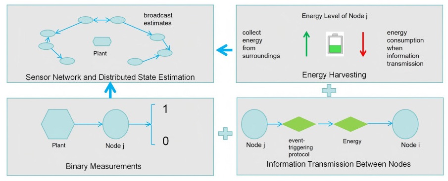
This paper addresses the distributed H∞-consensus state estimation issue for a class of discrete time-varying systems operating within binary sensor networks. An integral measurement output model is developed for each node to formulate the time intervals associated with sampling. Every binary sensor is equipped with an energy harvester to improve power efficiency. Information transmission between sensor nodes and their neighboring nodes is carefully orchestrated through a dynamic event-triggering protocol. Valuable information for estimation purposes is obtained by analyzing the discrepancies between the real and predicted inputs of binary sensors. Information from neighboring nodes is only transmitted when the node’s energy level is positive and the event-triggering condition is met. Two random variables are introduced to represent the energy level and the information from neighboring nodes to be received or not, respectively. Based on the available information, a distributed estimator is constructed for every binary sensor, and the expected performance constraints are given for the dynamic characteristics of estimation errors within a finite horizon. Sufficient conditions are constructed to obtain the desired distributed estimation performance constraint, and associated estimator gains are achieved by resolving the recursive linear matrix inequalities at each node, indicating the excellent scalability of the proposed approach. Ultimately, the effectiveness of the distributed estimation algorithm proposed in this paper is validated through an extensive simulation analysis.
Keywords
1. INTRODUCTION
In the past decades, wireless sensor networks have gained rapidly prominence in the tech world and have been widely adopted in a multitude of critical sectors[1], including target tracking[2], high-source localization[3], parameter identification[4], hazardous environment exploration[5], parabolic systems[6], and earthquake detection[7]. Sensor networks are generally made up of numerous sensor nodes that collaborate to observe specific regions and collect environmental information. As a new kind of estimation scheme, distributed estimation has been developed on the hardware basis of sensor networks. Scalable design has become a hot topic when studying the distributed estimation problem due to the large scale of sensor networks. In accordance with vector dissipation theory, the local performance analysis (LPA) method has been shown to be an effective tool to achieve scalable design of distributed estimation[8,9].
Due to their cost-effectiveness, binary sensor networks (BSNs) have garnered significant attention[10,11,12,13], resulting in greater focus on the estimation and control challenges associated with binary measurements (BMs)[14,15,16,17]. It is important to recognize that a single binary sensor can supply only a bit of data, which is inadequate for estimation purposes. To obtain meaningful insights from BM, an effective information extraction method has been proposed based on deterministic thresholds in[14,17]. The fundamental principle of this approach involves considering the binary sensor’s threshold as a weighted sum of two basis models. Then it leverages the discrepancy between the actual and predicted values to extract valuable insights. This method offers an effective means of acquiring valuable information from BM, thereby enhancing the estimation and control of the state of the system.
Most researchers implicitly assume that measurement outputs are functions of the system’s condition at the present time interval. Nevertheless, this presumption often falls short in real-world scenarios. Due to delayed data collection, system measurements are obtained within a given time interval, leading to the phenomenon of integral measurements. This phenomenon frequently occurs in processes such as chemical processes[18] and nuclear reactions[19]. Recently, the challenge of estimating integral measurements has started to attract research attention[20,21]. For example, state estimation and fault reconstruction schemes have been proposed in[20] in a specific category of discrete-time systems subject to partially decoupled disturbances. The state estimation problem has been studied by Shen et al.[21] for multirate artificial neural networks that incorporate integral measurements under the
In network control systems, limited bandwidth would result in signal transmission bottlenecks, which could give rise to various undesirable network-induced phenomena such as time delays, data collision, packet losses, etc.[22,23,24]. To mitigate the frequency of transmissions, an effective strategy is to implement the so-called event-triggering protocol (ETP), which operates on the principle of transmitting essential information solely when a predefined event-triggering condition is satisfied[27,26,25,28,29,30,31]. It should be noted that most existing ETPs are static, which implies that the threshold in event-triggering conditions cannot be adjusted. To optimize the utilization of communication resources, the concept of dynamic ETP has been introduced in previous works[32,34,33], which leverages non-negative internal variables to adaptively adjust the threshold parameters. Specifically, when it comes to resource-constrained wireless sensor networks, dynamic ETP has been applied by Ge et al.[33] to schedule local measurement transmissions between neighboring nodes to address distributed set-membership estimation problems.
In the realm of estimation problems, the core of consensus-based estimation schemes lies in fusing each node’s own estimation information with that received from its neighboring nodes and then transmitting this integrated estimation result to the entire estimation system. However, it should be noted that a crucial practical factor is often overlooked in most of the existing literature: the energy consumption required for information transmission between neighboring nodes[35,36,37]. In real-world applications, when sensor nodes directly transmit information, to sustain prolonged communication abilities, it is essential for sensors to discover efficient methods for energy restoration and effective energy replenishment. In recent years, energy harvesting (EH) technology has garnered significant research interest due to its sustainability and environmental benefits. This innovative approach has been successfully implemented in various industrial sectors[38,39].
For the filtering issues of EH sensors, the academic community has also achieved a series of promising research results[40,41,42,43]. However, the EH process is formulated by significant randomness, which directly leads to randomness in the amount of energy stored by sensors. In some cases, sensors may be unable to maintain communication with other sensors due to insufficient energy, thereby restricting communication and resulting in intermittent data transmission. Faced with this discontinuous communication mode, the analysis of transmission probability becomes particularly critical in the design of distributed estimators. Especially in distributed estimation, where multiple sensors are involved, the issue of energy consumption is particularly prominent. Therefore, introducing EH mechanisms into distributed estimation systems and proposing a novel estimation method that considers energy constraints for sensors with EH capabilities represent the main research motivation of this paper.
By summarizing the arguments so far, the key focus of our research lies in integrating the issues discussed above, particularly in scheduling dynamic ETPs to optimize the effectiveness of distributed state estimation utilizing EH. The key obstacles encountered in this procedure are detailed below: (1) How can we model dynamic ETPs, EH, and BMs within a unified framework? (2) Given the probability of energy availability, how can we leverage dynamic ETPs to derive an optimal transmission strategy? (3) To alleviate the computational load, what methods can we employ to define adequate conditions for
In response to the above challenging problems, the main innovations are summarized as three folds: (1) an LPA technique is proposed to address the distributed
The structure of the remaining part of this paper is outlined as follows. Section 2 elaborates on the problem to be studied, including the system, integral measurements, dynamic ETP, methods for BM information extraction, energy level parameter settings for EH sensors, the distributed estimator and the desired performance constraints. In Section 3, the required distributed estimation scheme is developed using the LPA method. Moreover, the estimator gains are derived by resolving a series of recursive linear matrix inequalities (RLMIs). Section 4 provides a case study to illustrate the effectiveness of the suggested distributed estimation method. In Section 5, the final conclusions are presented.
2. PROBLEM FORMULATION
2.1. Topology of sensor network
As for a BSN, its topology is formulated as a digraph
2.2. System formulations
Consider a state-space mode of discrete time-varying systems as follows:
where
The measurement of binary sensor
where
Regarding the integral measurements, the sample-state augmentation method (i.e., the lifting method) has been utilized to address integral measurements[18]. Subsequently, the lifting method has become a widely adopted approach for studying estimation problems involving integral measurements[44,45]. For integral measurement (2), denote
where
2.3. Distributed estimator for binary sensor
Construct a distributed estimator for binary sensor i using all the available information:
where
Now, introduce the principle of obtaining useful information for estimation purposes. From (2), (5) and (7), under the case of
where the uncertain scalar
By resorting to (8), one further has
According to (4),
2.4. Dynamic event-triggering protocol
This subsection uses a dynamic ETP to determine whether the neighbor’s information should be sent to node i at the current time. The event-triggering time sequence
where
and
where
In addition, to describe the effect of the dynamic ETP, define the following indicative variable as follows:
2.5. Energy harvesting
The inherent constraints in energy storage units within the sensors often prove inadequate for sustained information transmission between neighboring nodes. Consequently, our focus shifts to EH techniques, where a sensor, armed with an energy harvester, has the ability to harvest energy from the surrounding environment and convert it into electrical energy for the purposes of information transmission. Following a similar idea as in[47,48,46], the EH model is formulated for a neighboring node j of node i.
To begin with, the energy collected by the sensor node j is denoted by a random variable
where the integer b is the upper bound of the collected energy, and the scalar
Remark 1 Under certain assumptions, the energy harvested by sensor node j, which follows a binomial distribution, can be interpreted based on the principles of photovoltaic power generation. For simplicity, let b denote the total number of photons incident on a specific area of the material surface during the time interval from
Next, the energy level of the sensor node j
where
Here,
Remark 2 As introduced in the Introduction, EH and ETPs have been investigated for distinct underlying motivations. Specifically, EH is primarily motivated by the need to model the impact of energy consumption during information transmission. In contrast, the ETP aims to conserve energy by reducing the frequency of information transmissions through the imposition of a predefined triggering condition. In this paper, building upon existing results, we aim to investigate the precise energy-saving effect achieved within a framework that integrates both ETPs and EH techniques.
According to the previous analysis, the following distributed estimator is constructed:
2.6. Problem statement
Denoting
Letting
where
In the following, the system dynamics Equation 18 is provided with the specified performance metric.
Definition 1 For any node
The aim of this paper is to find the appropriate estimator gains, denoted as
3. MAIN RESULTS
3.1. Probabilistic distribution law of energy level
As discussed earlier, the transmission of information between neighboring nodes can only be achieved if the energy level is positive (that is,
Denote
Lemma 1. [43] The following conclusions hold
where
and
where
3.2. Vector dissipation
This subsection provides the LPA method to derive sufficient local conditions for any node
Let
Definition 2 It is said that the system dynamics Equation 18 is stochastic dissipative regarding the supply rate function
Furthermore, the system dynamics Equation 18 is vector dissipation regarding the vector supply rate function
Here, for any two vectors with the same dimensions,
Here, as the focus of the LPA method, Equation 23 refers to the vector dissipation inequality, which is constructed by seeking suitable local conditions of node
3.3. Scalable distributed state estimation scheme
For proceeding further, for any node
and choose the supply rate function:
where
With the help of the LPA method, a sufficient criterion regarding the performance constraint Equation 19 is established in the subsequent theorem for the system dynamics Equation 18 by means of the vector dissipation of system Equation 18 regarding the supply rate function
Theorem 1. Consider any binary sensor
Let
where
Proof 1. For node i, choose the scalar storage function with the following form:
where
Calculate the mathematical expectation of the storage function along the dynamics of Equation 12 and Equation 19
where
In addition, we also obtain
According to Equation 15, we introduce a positive scalar
As such, one further has
which implies that
Then, in light of Equation 29, one immediately has
where
Moreover, since
By means of the double expectation theorem, one obtains that
which can be rewritten in a compact form:
Next, a scalar form is derived by making the linear transformation to Equation 32:
which is further calculated in light of the property of dissipation matrix W as follows:
Furthermore, the above inequality can be rewritten as
Next, Equation 34 is summed regarding u from
which indicates that
Noticing that
and, therefore, one has Equation 19 according to
Furthermore, denoting
In the following, the desired estimator gains are calculated in terms of recursive linear matrix inequalities by resorting to the Schur Complement Lemma.
Theorem 2. Consider any binary sensor
Let
where
Furthermore, if Equation 38 is feasible, then one calculates
Proof 2. By resorting to the Schur Complement Lemma, it follows that Equation 25holds if and only if
Next, the left-hand side of Equation 39 is partitioned as
where
Next, one acquires the following compact form
where
By means of S-Procedure,
By reusing Schur Complement Lemma, Equation 42 holds if and only if
where
After performing the congruent transformation
Remark 3 colorblueIt should be noted that Theorems 1 and 2 provide the parameter constraints that are helpful in achieving the desirable performance constraint and reproducing the results and understanding the engineering implications of the model.
Remark 4 The scalable distributed
4. AN ILLUSTRATIVE EXAMPLE
In this section, a demonstrative example is provided to show the efficiency and viability of the proposed distributed
The topology structure of BSN is depicted by the digraph
The system parameters in Equation 1 and Equation 2 is chosen as follows:
The sensor parameters are set as
The initial values are set as
The energy harvester parameters for every node are set as
By means of Lemma 1, one then has
Figures 1-8 plot all simulation results under Case Ⅰ. More specifically, Figure 1 and Figure 2 depict the true state and its estimations from each binary sensor under the dynamic ETP and EH; Figure 3 plots the time instants of
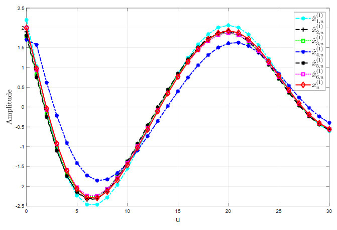
Figure 1. xu(1) and its estimates under case Ⅰ.
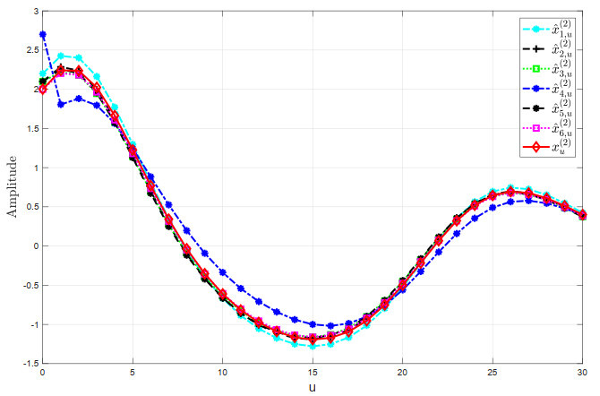
Figure 2. xu(2) and its estimates under case Ⅰ.
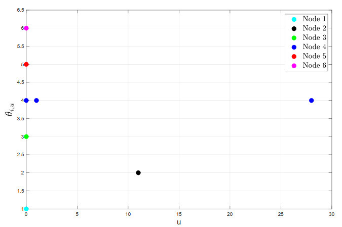
Figure 3. The time instants of
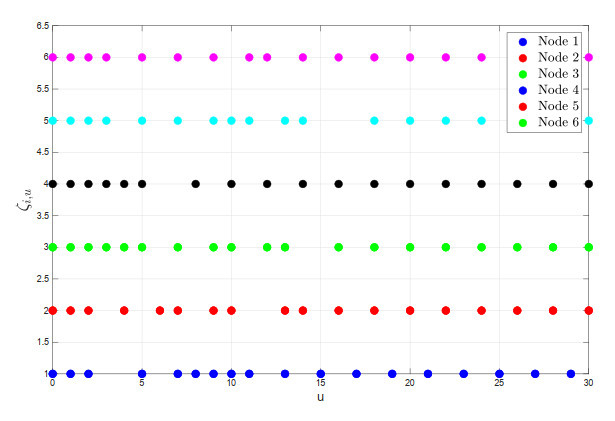
Figure 4. The information transmission instants under case Ⅰ.
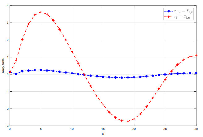
Figure 5.
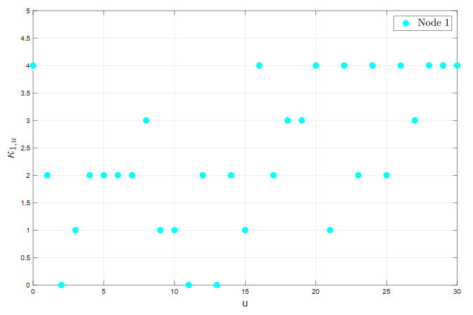
Figure 6. Energy level of node 1 under case Ⅰ.
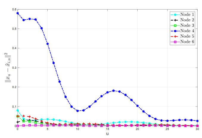
Figure 7.
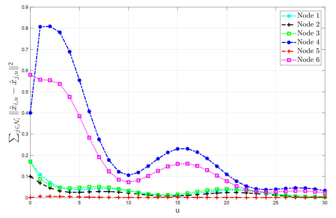
Figure 8.
It follows from Figure 6 that the dynamic change in the amount of energy inside the sensor depends on both the communication consumption and the generation of EH. In light of Figure 3, at certain time instants, the useful information from every binary sensor is extracted for estimation purposes in light of Equation 5 and Equation 6. According to Figure 4, due to the introduction of dynamic ETP, the transmission frequency of the six nodes in the sensor network decreases significantly, and the triggering frequency of the transmission of information also decreases with time, further saving network resources. According to Figure 5, it is relatively small of the differences between
From Figure 1 and Figure 2, it follows that despite the limitations imposed by the energy harvester and dynamic ETP, the estimation of each binary sensor maintains a commendable level of accuracy in discerning the actual state. As depicted in Figure 7 and Figure 8, both the estimation errors and the consensus errors of every binary sensor meet the aspired performance criteria.
Next, consider Case Ⅱ: the dynamic ETP without energy constraints. To this end, we set
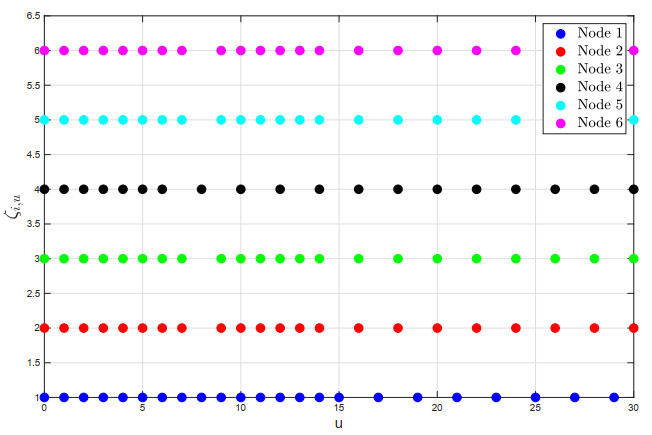
Figure 9. Information transmission time instants under case Ⅱ.
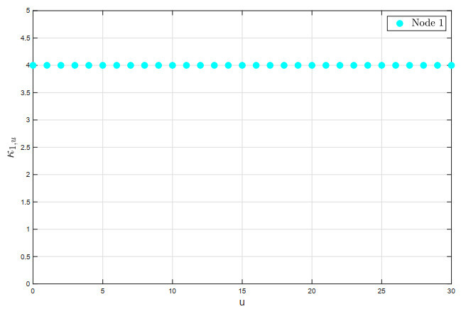
Figure 10. Energy level of node 1 under case Ⅱ.
Next, consider Case Ⅲ: the static ETP without energy constraints, i.e.,
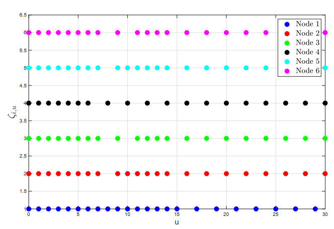
Figure 11. Information transmission time instants of node 1 under case Ⅲ.
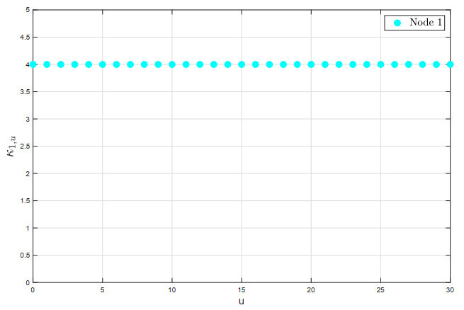
Figure 12. Energy level of node 1 under case Ⅲ.
Finally, consider Case Ⅳ: the scenario with only an energy constraint but no ETP, i.e.,
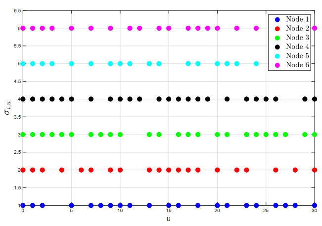
Figure 13. Information transmission time instants of node 1 under case Ⅳ.
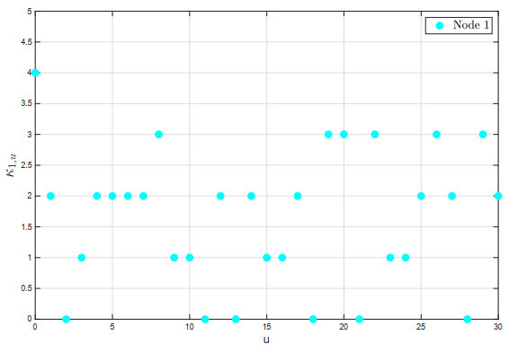
Figure 14. Energy level of node 1 under case Ⅳ.
In conclusion, the simulations collectively demonstrate the desirable performance of the proposed distributed
5. CONCLUSIONS
This paper has proposed a distributed state estimation scheme using integral measurements in BSNs, considering the EH technique and dynamic ETP. A new BM model has been established for each node by choosing the integral measurements as inputs of the BMs. The random variable obeying the binomial distribution has been used to describe energy levels and an indicator variable has been introduced to formulate the effect of dynamic ETP. The dynamic ETP and EH methods have been used cooperatively for each node to decide whether information should be transmitted from its neighboring nodes. Based on the available information, distributed consensus estimators have been constructed for each sensor. Through the LPA method, sufficient conditions have been established for each node to ensure that the estimation error of all nodes meets the desired
DECLARATIONS
Authors’ contributions
Conceptualization and manuscript drafting: Han, F.; Ma, L.
Methodology and experiment: Song, Y.
Manuscript edition: Zhang, J.
Review and supervision: Shao, S.
Availability of data and materials
The authors generated all data and materials used in the research as an integral part of the study, with explicit details provided in the methodology section of the manuscript. These are available from the corresponding author upon reasonable request.
AI and AI-assisted tools statement
Not applicable.
Financial support and sponsorship
This work was supported in part by the National Natural Science Foundation of China under Grant Nos. U21A2019, U24B6004, and 62073070, and by the Natural Science Foundation of Heilongjiang Province of China under Grant No. LH2024F006.
Conflicts of interest
All authors declared that there are no conflicts of interest.
Ethical approval and consent to participate
Not applicable.
Consent for publication
Not applicable.
Copyright
© The Author(s) 2026.
REFERENCES
1. Wang, Y. A.; Shen, B.; Zou, L.; Han, Q. L. A survey on recent advances in distributed filtering over sensor networks subject to communication constraints. Int. J. Netw. Dyn. Intell. 2023, 2, 100007.
2. Guo, J.; Zhang, J. F.; Zhao, Y. Adaptive tracking of a class of first-order systems with binary-valued observations and fixed thresholds. J. Syst. Sci. Complex. 2012, 25, 1041-51.
3. Bai, E. W. Source localization by a binary sensor network in the presence of imperfection, noise and outliers. IEEE. Trans. Autom. Control. 2018, 63, 347-59.
4. Wang, Y.; Zhao, Y.; Zhang, J. F. Distributed recursive projection identification with binary-valued observations. J. Syst. Sci. Complex. 2021, 34, 2048-68.
5. Yick, J.; Mukherjee, B.; Ghosal, D. Wireless sensor network survey. Comput. Netw. 2008, 52, 2292-330.
6. Qian, X.; Cui, B. A mobile sensing approach to distributed consensus filtering of 2D stochastic nonlinear parabolic systems with disturbances. Syst. Sci. Control. Eng. 2023, 11, 2167885.
7. Hu, Z.; Hu, J.; Tan, H.; Huang, J.; Cao, Z. Distributed resilient fusion filtering for nonlinear systems with random sensor delay under Round-Robin protocol. Int. J. Syst. Sci. 2022, 53, 2786-99.
8. Han, F.; Wang, Z.; Liu, H.; Dong, H.; Lu, G. Local design of distributed state estimators for linear discrete time-varying systems over binary sensor networks: a set-membership approach. IEEE. Trans. Syst. Man. Cybern. Syst. 2024, 54, 5641-54.
9. Han, F.; Wang, Z.; Liu, H.; Dong, H.; Lu, G. A recursive matrix inequality approach to distributed filtering over binary sensor networks: handling amplify-and-forward relays. IEEE. Trans. Netw. Sci. Eng. 2024, 11, 1347-62.
10. Ciuonzo, D.; Aubry, A.; Carotenuto, V. Rician MIMO channel-and jamming-aware decision fusion. IEEE. Trans. Signal. Process. 2017, 65, 3866-80.
11. Jin, Y.; Ma, X.; Meng, X.; Chen, Y. Distributed fusion filtering for cyber-physical systems under Round-Robin protocol: a mixed H2/H∞ framework. Int. J. Syst. Sci. 2023, 54, 1661-75.
12. Mousavinejad, E.; Ge, X.; Han, Q. L.; Lim, T. J.; Vlacic, L. An ellipsoidal set-membership approach to distributed joint state and sensor fault estimation of autonomous ground vehicles. IEEE-CAA. J. Automatica. Sin. 2021, 8, 1107-18.
13. Su, Y.; Cai, H.; Huang, J. The cooperative output regulation by the distributed observer approach. Int. J. Network. Dyn. Intell. 2022, 1, 20-35.
14. Battistelli, G.; Chisci, L.; Forti, N.; Gherardini, S. MAP moving horizon state estimation with binary measurements. Int. J. Adapt. Control. Signal. Process. 2020, 34, 796-811.
15. Hu, Z.; Chen, B.; Zhang, Y.; Yu, L. Kalman-like filter under binary sensors. IEEE. Trans. Instrum. Meas. 2022, 71, 9503111.
16. Wang, T.; Zhang, H.; Zhao, Y. Consensus of multi-agent systems under binary-valued measurements and recursive projection algorithm. IEEE. Trans. Autom. Control. 2020, 65, 2678-85.
17. Zhang, Y.; Chen, B.; Yu, L. Fusion estimation under binary sensors. Automatica. 2020, 115, 108861.
18. Guo, Y.; Huang, B. State estimation incorporating infrequent, delayed and integral measurements. Automatica. 2015, 58, 32-8.
19. Casoli, P.; Authier, N.; Jacquet, X.; Cartier, J. Characterization of the caliban and prospero critical assemblies neutron spectra for integral measurements experiments. Nucl. Data. Sheets. 2014, 118, 554-7.
20. Liu, Y.; Wang, Z.; Zhou, D. State estimation and fault reconstruction with integral measurements under partially decoupled disturbances. IET. Control. Theory. Appl. 2018, 12, 1520-6.
21. Shen, Y.; Wang, Z.; Shen, B.; Alsaadi, F. E. H∞ state estimation for multi-rate artificial neural networks with integral measurements: a switched system approach. Inf. Sci. 2020, 539, 434-46.
22. Caballero-Águila, R.; Hermoso-Carazo, A.; Linares-Pérez, J. Networked fusion estimation with multiple uncertainties and time-correlated channel noise. Inf. Fusion. 2020, 54, 161-71.
23. Hu, J.; Zhang, H.; Yu, X.; Liu, H.; Chen, D. Design of sliding-mode-based control for nonlinear systems with mixed-delays and packet losses under uncertain missing probability. IEEE. Trans. Syst. Man. Cybern. Syst. 2021, 51, 3217-28.
24. Pang, Z. H.; Fan, L. Z.; Dong, Z.; Han, Q. L.; Liu, G. P. False data injection attacks against partial sensor measurements of networked control systems. IEEE. Trans. Circuits. Syst. Ⅱ. 2022, 69, 149-53.
25. Sun, Y.; Tian, X.; Wei, G. Finite-time distributed resilient state estimation subject to hybrid cyber-attacks: a new dynamic event-triggered case. Int. J. Syst. Sci. 2022, 53, 2832-44.
26. Qu, F.; Zhao, X.; Wang, X.; Tian, E. Probabilistic-constrained distributed fusion filtering for a class of time-varying systems over sensor networks: a torus-event-triggering mechanism. Int. J. Syst. Sci. 2022, 53, 1288-97.
27. Li, X.; Ye, D. Dynamic event-triggered distributed filtering design for interval type-2 fuzzy systems over sensor networks under deception attacks. Int. J. Syst. Sci. 2023, 54, 2875-90.
28. Cao, J.; Ding, D.; Liu, J.; Tian, E.; Hu, S.; Xie, X. Hybrid-triggered-based security controller design for networked control system under multiple cyber attacks. Inf. Sci. 2021, 548, 69-84.
29. Song, W.; Wang, J.; Wang, C.; Shan, J. A variance-constrained approach to event-triggered distributed extended Kalman filtering with multiple fading measurements. Int. J. Robust. Nonlinear. Control. 2019, 29, 1558-76.
30. Wei, G.; Liu, L.; Wang, L.; Ding, D. Event-triggered control for discrete-time systems with unknown nonlinearities: an interval observer-based approach. Int. J. Syst. Sci. 2020, 51, 1019-31.
31. Zhang, P.; Yuan, Y.; Guo, L. Fault-tolerant optimal control for discrete-time nonlinear system subjected to input saturation: a dynamic event-triggered approach. IEEE. T. Cybern. 2021, 51, 2956-68.
32. Ju, Y.; Tian, X.; Liu, H.; Ma, L. Fault detection of networked dynamical systems: a survey of trends and techniques. Int. J. Syst. Sci. 2021, 52, 3390-409.
33. Ge, X.; Han, Q. L.; Wang, Z. A dynamic event-triggered transmission scheme for distributed set-membership estimation over wireless sensor networks. IEEE. T. Cybern. 2019, 49, 171-83.
34. Liu, Y.; Shen, B.; Shu, H. Finite-time resilient H2 state estimation for discrete-time delayed neural networks under dynamic event-triggered mechanism. Neural. Netw. 2020, 121, 356-65.
35. Liu, L. N.; Yang, G. H. Distributed energy resource coordination for a microgrid over unreliable communication network with DoS attacks. Int. J. Syst. Sci. 2024, 55, 237-52.
36. Dong, S. S.; Li, Y. G.; An, L. Optimal strictly stealthy attacks in cyber-physical systems with multiple channels under the energy constraint. Int. J. Syst. Sci. 2023, 54, 2608-25.
37. Zhao, Z.; Xia, L.; Jiang, L.; Ge, Q.; Yu, F. Distributed bandit online optimisation for energy management in smart grids. Int. J. Syst. Sci. 2023, 54, 2957-74.
38. Pehlivan, I.; Ergen, S. C. Scheduling of energy harvesting for MIMO wireless powered communication networks. IEEE. Commun. Lett. 2019, 23, 152-5.
39. Sudevalayam, S.; Kulkarni, P. Energy harvesting sensor nodes: Survey and implications. IEEE. Commun. Surv. Tutor. 2011, 13, 443-61.
40. Hentati, A.; Frigon, J. F.; Ajib, W. Energy harvesting wireless sensor networks with channel estimation: Delay and packet loss performance analysis. IEEE. Commun. Surv. Tutor. 2020, 69, 1956-69.
41. Knorn, S.; Dey, S.; Ahlén, A.; Quevedo, D. E. Optimal energy allocation in multisensor estimation over wireless channels using energy harvesting and sharing. IEEE. Trans. Autom. Control. 2019, 64, 4337-44.
42. Leong, A. S.; Dey, S.; Quevedo, D. E. Transmission scheduling for remote state estimation and control with an energy harvesting sensor. Automatica. 2018, 91, 54-60.
43. Shen, B.; Wang, Z.; Tan, H.; Chen, H. Robust fusion filtering over multisensor systems with energy harvesting constraints. Automatica. 2021, 131, 109782.
44. Zhu, X.; Liu, Y.; Fang, J.; Zhong, M. Fault detection for a class of linear systems with integral measurements. Sci. China. Inf. Sci. 2021, 64, 132207.
45. Shen, Y.; Wang, Z.; Dong, H.; Alsaadi, F. E.; Liu, H. Dynamic event-based recursive filtering for multirate systems with integral measurements over sensor networks. Int. J. Robust. Control. 2021, 32, 1374-92.
46. Li, Y.; Zhang, F.; Quevedo, D. E.; Lau, V.; Dey, S.; Shi, L. Power control of an energy harvesting sensor for remote state estimation. IEEE. Trans. Autom. Control. 2017, 62, 277-90.
47. Chen, W.; Wang, Z.; Ding, D.; Yi, X.; Han, Q. L. Distributed state estimation over wireless sensor networks with energy harvesting sensors. IEEE. T. Cybern. 2023, 53, 3311-24.
48. Huang, J.; Shi, D.; Chen, T. Event-triggered state estimation with an energy harvesting sensor. IEEE. Trans. Autom. Control. 2017, 62, 4768-75.
49. Zou, L.; Wang, Z.; Shen, B.; Dong, H. Secure recursive state estimation of networked systems against eavesdropping: a partial-encryption-decryption method. IEEE. Trans. Autom. Control. 2025, 70, 3681-94.
Cite This Article
How to Cite
Download Citation
Export Citation File:
Type of Import
Tips on Downloading Citation
Citation Manager File Format
Type of Import
Direct Import: When the Direct Import option is selected (the default state), a dialogue box will give you the option to Save or Open the downloaded citation data. Choosing Open will either launch your citation manager or give you a choice of applications with which to use the metadata. The Save option saves the file locally for later use.
Indirect Import: When the Indirect Import option is selected, the metadata is displayed and may be copied and pasted as needed.
About This Article
Copyright

Data & Comments
Data
0


Comments
Comments must be written in English. Spam, offensive content, impersonation, and private information will not be permitted. If any comment is reported and identified as inappropriate content by OAE staff, the comment will be removed without notice. If you have any queries or need any help, please contact us at [email protected].